


Back-of-the-envelope calculations are useful at the beginning of a project for estimating LED type and count. This article presents techniques for calculating optical quantities and estimating LED count for some typical applications.
Optical principles
Before any calculations can be started, a basic understanding of optical principles must be established. The principles most important for solid state lighting (SSL) applications are reflection, refraction and total internal reflection (TIR).
Reflection
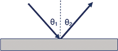
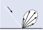
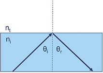
The law of reflection states that for a ray striking a reflective surface, the angle of incidence is equal to the angle of reflection (see Figure 1). A reflection that obeys this law is called a specular reflection. If the reflective surface has some roughness (which is always the case), some portion of the incident light will be reflected at some angle other than the specular angle of reflection. In the extreme condition, the reflective surface is perfectly diffuse and the reflected light scatters in all directions. In practice, reflections are somewhere between perfectly specular and perfectly diffuse (see Figure 2). Light passing through a surface can also be diffusely transmitted.
Refraction
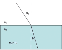
When light passes from one media into another (say, from air to plastic), it is bent (changes direction). The angle of this change in direction follows Snell’s Law, which is:
n1 sinθ1 = n2 sinθ2,
where n1 and n2 are the indices of refraction of the two media, θ1 is the angle of incidence, and θ2 is the angle of the refracted ray (see Figure 3).
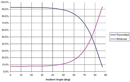
At every interface between two media, some of the light will be transmitted (refracted) and some will be reflected. In the case of a lens, the reflected light is considered to be lost. This is called Fresnel loss or Fresnel reflection and is dependent upon the indices of refraction of the two media and the angle of incidence. Figure 4 shows how these losses vary with angle of incidence. As evident from the chart, these losses become significant at around 60° for plastic.
Total internal reflection (TIR)
When light is passing from a more dense medium to a less dense medium (greater index to lesser index, such as plastic to air), the change in angle obeys Snell’s Law. However, as the angle of incidence increases, there comes a point where the light does not escape the plastic and the air-plastic interface acts as a mirror. This phenomenon is called total internal reflection (TIR). The angle at which this occurs is called the critical angle and depends upon the two materials (see Figure 5). Because the reflection is lossless (free of Fresnel losses), high efficiency optics can be designed which make use of this principle.
Optical quantities
Radiometric quantities refer to optical radiation in general. Photometric quantities are the radiometric quantities weighted to the response of the human eye. For visible lighting applications, only photometric quantities will be used.
Radiometric and photometric quantities
For visible applications, we are typically concerned with luminous flux, luminous intensity, illuminance and luminance.
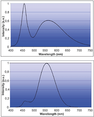
Conversion from radiometric Watts to photometric lumens is accomplished by the equation
where S(λ) is the radiometric spectrum, V(λ) is the response curve of the eye, and K is a constant. Figure 6 shows the spectra of a white LED in radiometric and photometric units.
Luminous flux has units of lumens and is a measure of optical power. OSRAM Opto Seminconductors’ LEDs for SSL applications are binned by luminous flux. Most optical calculations seek to discover how many source lumens (and therefore, number of LEDs) are required for an application.
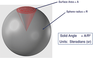
Luminous intensity (or simply intensity) is the amount of light in a direction. Its units are lumens per unit solid angle (in steradians), or candela. The concept of solid angle is illustrated in Figure 8.
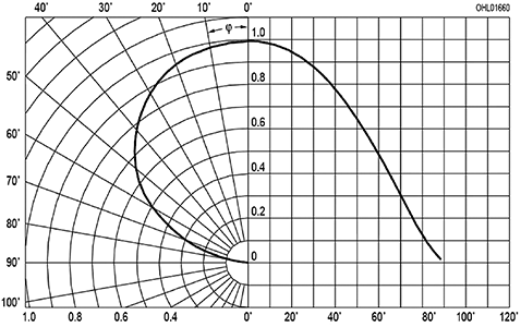
Historically, most high-power LEDs have a nearly Lambertian intensity distribution, i.e. I = I0cosθ (see Figure 9). Besides Lambertian, OSRAM Opto Semiconductors’ LEDs come in a variety of intensity distributions designed to suit specific applications (see Figure 10).
Illuminance is the amount of light falling on a surface and has units of lumens per unit area. Metric units are lux (lumens per square metre), while English units are foot-candles (lumens per square foot). An important concept related to illuminance is the inverse-square law
where I = intensity of the source and R = distance from the source. Downlights are specified by their centre beam intensity and illuminances at different distances.
Luminance is the amount of light from a surface in a direction. It is lumens per projected solid angle per area, and is typically measured in candela per square metre, or Nits. Luminance is what the eye detects; when people talk about the ‘brightness’ of a light, they are actually describing luminance.
Optical loss factors
In order to calculate the number of lumens (and therefore, number of LEDs) for an application, the losses in the optical system must be accounted for. These include the collection efficiency (how much of the initial light is directed in a useful direction), and reflection and transmission losses (due to Fresnel losses and absorption). Table 1 summarises some rule-of-thumb loss factors for various optical elements (the loss factors were collected from several suppliers of off-the-shelf optics).
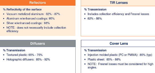
For reflectors, it is necessary to consider the reflectivity of the surface and its collection efficiency. The reflectivity is only applied to the light that actually strikes the reflector. Aluminium coated plastic reflectors are common, and their reflectivity is typically in the range of 82%-87% depending on how well the plastic is moulded and how well the aluminium coating is applied. For a first estimate, a value of 85% can be used.
It should be noted that white reflectors can have comparable values for reflectivity, but the reflections will be less specular. The spectrum of the light and spectral reflectivity of the white material also become important. The loss factor of TIR lenses includes the collection efficiency and Fresnel losses at the entrance and exit interfaces. Off-the-shelf optics typically have loss factors ranging from 82%-88%. A value of 85% is typical for a first estimate.
Refractors (lenses) and flat cover lenses are similar to reflectors in terms of their loss factors. An imaging lens can only collect a portion of the LED light. It will also have transmission loss due to Fresnel loss and manufacturing tolerances.
Because of their higher efficiencies, TIR lenses are generally preferred for SSL applications.
For many applications, a cover lens is added for protection from the environment. Even a flat lens will have Fresnel losses and manufacturing losses.
A cover lens with a contoured shape can have a transmission of 85%. Flat plastic sheets tend to be higher, in the range of 85%-88%. It is also important to remember that Fresnel losses can become significant for high angles of incidence.
Sometimes, a diffuser is added to the system to increase the uniformity of the lit appearance or the output beam. This could be anything from texturing the cover lens to using a holographic diffuser. Transmission losses can vary greatly, so some idea of what specific diffuser will be used is necessary for making calculations.
Application case studies
Two case studies will be used to help illustrate the calculations. The first is a streetlight application based upon an actual project. The second is an idealised downlight.
Streetlight LED retrofit
This was a demonstration project using an existing luminaire. The project parameters were as follows:
• LED: OSRAM Opto Semiconductors OSLON 80
• Number of LEDs: 66
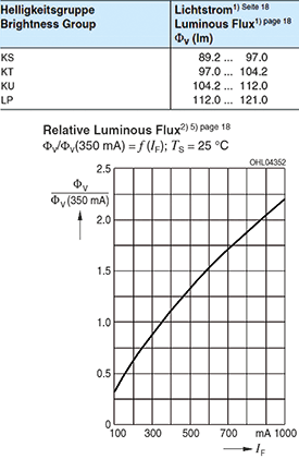
• Source lumens per LED: 112 lm
• Optical system: stock TIR lenses (1 per LED).
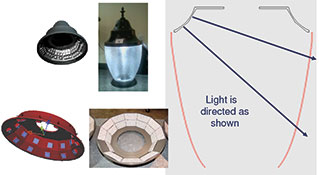
The optics and LEDs were mounted on PCBs, each of which were aimed in a particular direction to achieve the final beam pattern.
The question is: how many lumens can be expected on the ground? Lifetime, power consumption, and cost considerations led to constraints on the number of LEDs and the drive current. The number of LEDs was known to be 66, and the source lumens were expected to be 112 based upon the expected flux bin and drive current. Additional optical losses were expected from the cap and the base (see Figure 11).

The optic loss factor is the efficiency of the TIR optic. The outer lens loss factor is set at 85% since the Fresnel losses are not expected to be high. The amount of light blocked by the cap and lamp base (blocked light loss factor) is unknown, but (hopefully) should be small; a 10% loss is assumed.
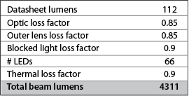
One important non-optical loss factor needs to be included, and that is thermal degradation. As the LED gets hotter, its light output drops. The thermal degradation depends on the LED junction temperature (Tj), which in turn depends upon ambient temperature, LED power, and thermal management system (PCB, heatsink, fans, etc.). A junction temperature target of 70°C is assigned in order to meet the LED lifetime goal. From the datasheet, for a Tj of 70°C, the thermal loss factor is 0,9. With this additional factor, the calculation of total beam lumens is shown in Table 2.
When the prototype was built and measured, the actual beam lumens came out to 4403, which is very close to the estimate considering all the assumptions that were made.
Indoor downlight
Consider a downlight with a known maximum centre beam candlepower (MCBCP). What is the illuminance, in foot-candles, at different mounting heights? The units ‘candlepower’ are equivalent to ‘candela’. Both are measurements of intensity, in lumens per steradian. To solve this problem, we use the inverse square law equation
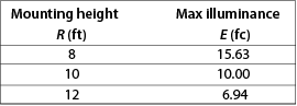
Using MCBCP = 1000 cd, Table 3 shows illuminance for different mounting heights. For a second example, assume the mounting height, area to be illuminated, and average illuminance are known. How many warm white Oslon LEDs (LCW CP7P) will be needed assuming secondary optics and a cover lens are used?
The sketch in Figure 12 illustrates the application and the equation needed for the calculation.
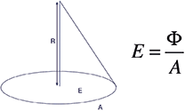
For the optical system, assume TIR optics are used to shape the beam, and a clear cover lens is also present. The calculations are shown in Table 4. The required lumens in area A are calculated using the equation in the sketch. The required source lumens are the required lumens in area A divided by the three loss factors.
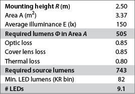
Finally, the number of LEDs is the required source lumens divided by the minimum lumens per LED. For the purposes of this calculation, flux bin KR is assumed. From the datasheet, the minimum lumens in this bin is 82.
Conclusion
Making back-of-the-envelope calculations for LED lighting requires only a basic understanding of the optical concepts and some typical loss factor values. While these initial calculations are useful, more detailed analysis using simulation software and prototypes can lead to reductions in LED count and design complexity.
For more information contact Michael Nel, OSRAM Opto Semiconductors, +27 (0)79 525 1779, m.nel@osram-os.com, www.osram-os.com


© Technews Publishing (Pty) Ltd | All Rights Reserved
 printer friendly version