


The first part of this article, covering the fundamental principles of GPS clock frequency disciplining, was published in the 11 October 2017 issue of Dataweek. This second and final part covers the ins and outs of holdover.
Holdover introduction
Although GNSS (global navigation satellite system) signals ‘rain’ from the sky, they are quite faint, have poor penetration and are easily obscured. They are not available (or reliable) indoors, in ‘urban canyons’ or noisy RF environments, so being able to hold the last known frequency and timing (phase) during a GNSS outage becomes a necessary requirement. This is why GNSS receivers are paired with high-quality oscillators, to create clock sources with holdover characteristics that can bridge temporary RF outages.
Unfortunately, those obscured places are the ones we need to run tests at (shielded cabinets, containers, base stations, central offices, equipment rooms, office buildings, basements, etc.). The proposed solution is to extend the use of holdover into becoming a temporary means of transporting time synchronisation from outdoors to indoors.
Before jumping into the holdover-for-testing explanation, keep in mind that the phase disciplining process constantly changes the oscillator’s frequency to keep its 1PPS aligned to the standard UTC second. Even though those fine adjustments are in the order of parts-per-trillion, they will affect the final holdover performance.
Using disciplining and holdover in actual field test applications
Figure 1 depicts the full time error (TE) cycle of a test set’s internal 1PPS reference, starting from free running, disciplining, to holdover. A relatively short holdover behaviour was selected as an example, so all the different phases can be easily visualised.
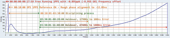
The test was run in conditions similar to what field technicians would encounter at remote sites. The main difference is that we had access to a 1PPS reference (PRTC) and equipment to monitor and document the internal 1PPS behaviour for this article, but field technicians won’t have the same luxury. That is the reason why it is important to carry reliable test instruments that provide as much information about their internal status and readiness as possible.
A test set, equipped with GPS receiver and chip-scale atomic clock oscillator, was selected for the experiment. It was turned on and its internal GPS-disciplined 1PPS reference was constantly recorded, but that extra TE information was not used for any decision making during the test. Let’s interpret this graph one section at a time.
Free running stage
The initial part of the trace in Figure 2 shows the internal 1PPS phase compared to the reference, while the GPS disciplining function was still disabled (free running). The first 1085 seconds of the TE trace indicate that the oscillator is very stable (straight line) but it has a free-run accuracy or frequency offset (ramp trend) of 0,895 ppb, which causes the phase to drift at a rate of 0,895 ns/s.
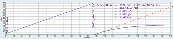
The straight TE lines, which identify highly stable oscillators, make it easier to measure its frequency offset by using simple math to calculate the slope (Y/X or TE/t). Modern test sets can also perform the offset calculation on their own, with the advantage that they can do it for more complex scenarios.
Disciplining process
18 minutes later (1085 seconds) the GPS (already locked to satellites) is enabled, to get the disciplining process started. The first thing that happens is the internal 1PPS being forced to align with the 10 MHz cycle closest to the UTC second. In this case, the TE reads -12,5 ns.
The first dot in Figure 3 shows a trend indicating that the internal oscillator still wants to run at 10 000 000,00895 Hz (10 MHz +0,895 ppb), after the initial rough phase correction. The disciplining control system starts to steer the oscillator into running slower and at the 2000 s mark it reaches exactly 10 000 000 Hz (0,0 ppb).
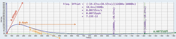
If the goal was to achieve frequency accuracy only, the process could have been stopped at this point and allowed to stay in that perfectly horizontal trend indicated by the dotted line. But the priority is phase (time) alignment and 300 ns error has accumulated in the process of getting to this point, which still needs to be corrected. So, the process continues by making the oscillator run a little bit slower than its ideal frequency, in order to make the pulse’s phase drift to the ‘left’, to reduce the phase error.
The third dot (at 3000 s) shows the oscillator running at 9 999 999,998715 Hz (-0,1285 ppb). As the 1PPS phase error approaches 0,0 ns, the oscillator starts to run a bit faster to make it converge. Depending on the conditions and settings, the whole process may take a long time, which could be an issue for field testing if not done correctly.
The fourth dot (at 12 600 s or 03:30:00) shows the oscillator running at around 10 000 000,0000715 Hz (0,00715 ppb), before the GPS 1PPS reference was disconnected. That is two orders of magnitude better than its free-running frequency.
At first this may look impressive, but even in a controlled lab environment a 0,00715 ns/s phase drift rate would cause the accumulation of 100 ns error in about 13 986 s (03:53:06).
Also note that, after checking the internal phase graph to confirm that the disciplining process has stabilised, the point of disconnection is basically selected at random (by a human). No one can really guarantee what the exact residual frequency offset is at every single occasion. It could be slightly larger or smaller, positive or negative, so there is a degree of uncertainty in the resulting holdover behaviour.
Keep in mind that field technicians don’t have access to some of the measurements or calculations shown here, when making the decision to force the test set (or external reference) into holdover, so having clear information about the internal disciplining process and status becomes very important.
Forcing the test set into holdover
At the 12,600 s mark the GPS was disabled (Figure 4), to force the test set’s internal 1PPS reference into holdover mode, so one can enter the premises to perform absolute time error, wander or one-way latency measurements.
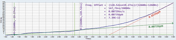
At 0,00739 ns/s phase drift rate, the initial trend is very close to what was calculated before the holdover started. This confirms that the oscillator will keep the last frequency correction to try holding the last known time. The first 100 ns error is accumulated after 17 900 s (04:58:20) of holdover and the 1000 ns threshold is reached after 47 400 s (13:19:00). Note that the oscillator’s frequency starts to drift a bit at the end of the day (5:45 pm or 10:19 am+34 000 s), due to significant drop in ambient temperature (winter). Nonetheless, it covered the regular working hours. This effect would be less noticeable in equipment rooms with continuous air conditioning (HVAC).
Repeatability
GPS-disciplined frequency references have an advantage in that their frequency correction factor (steer) can be measured, stored and re-applied later on, as long as the oscillator’s frequency retrace remains the same every time it is turned on. That is not the case for phase references, as they must remain powered in order to keep time. The selected phase reference must be battery powered in order to be used in field applications.
It is also important to know how the selected portable or built-in GNSS-disciplined clock source performs, under the conditions specific to a network and its environment. As mentioned before, the total holdover time to some amount of allowed uncertainty (or error) is mainly determined by (a) the frequency offset of the oscillator at the moment the GPS 1PPS is disabled or disconnected, (b) the stability of the oscillator, (c) temperature variations and (d) phase noise.
Once a good disciplined oscillator has been properly steered into parts-per-trillion accuracy, the point at which the GPS is disconnected could be one of the most important factors in determining how long the holdover would be. It is all about the frequency offset and temperature stability from that point on. Each time the same procedure is run, the results could be slightly different.
A week later, the same test set was used to run the experiment again, using approximately the same times to start the disciplining process and force the holdover. Figure 5 shows the differences between the first (blue) and second (red) tests. Temperature and sky conditions were slightly different since the second test was performed on a rainy day. That is a good example of what real-life field conditions mean.
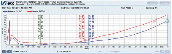
As expected, the two traces are slightly different. There is a baseline offset of about 70 ns between the original and the new TE traces, which could be due to the internal GPS clock plus the external GPS-disciplined reference uncertainties. Also, in the new test results (red) the first 100 ns accumulate faster (25 minutes earlier) and reaches the 1000 ns mark earlier, after 42 000 s of holdover.
If 100 ns uncertainty is considered acceptable, it could be said that such holdover reference could be used for up to four hours in both cases. It is important for field users to be aware that disciplined oscillators don’t behave exactly the same every time. At the same time one can’t assume that holdover performance is always that short. The better you know the basic theory and the instruments, the more reliable the holdover performance would be.
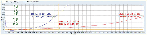
If the same test is run again, carefully applying all the guidance provided in this article, the performance can improve significantly, as shown by the results in Figure 6. In this last example (red), the test set runs for more than 13 hours before accumulating 100 ns error and it takes more than 43 hours to accumulate 1000 ns error – significantly better than the original (blue) one, and it was also a field test (not a controlled lab test). As we all learn from true field experiences, test and measurement vendors may be able to automate part of the holdover initiation process to guarantee the best holdover possible under given conditions.
It is technically possible to correct phase drift effects due to frequency offset to improve repeatability. The linear phase drift effects (stable frequency offset) can be measured with great precision and mathematically removed, but it could be cumbersome and/or too expensive for field testing.
Some experts suggest having a GPS-disciplined time reference in the vehicle, which could be used at the beginning and at the end of each test to measure the instrument’s internal 1PPS drift, calculate the frequency offset associated with it and mathematically removing its contribution from the recorded data. This could be an expensive proposition and it requires users to run outside after every test to measure the error accumulated by the portable reference.
A simpler approach may be to make users go outside after every test, and resync to GPS so the instrument can measure its accumulated phase error, calculate its phase drift rate and apply a (linear) mathematical correction to the recorded TE data. It is technically possible today, but the running outside part still needs some consideration.
Portability and battery operation
The use or need for extended holdover in test and measurement implies battery backup, at least to keep the internal clock ticking while the instrument is being transported to the test site. Since holdover degrades timing accuracy over time, it is best if the test set can be disciplined on site (e.g. via GPS) to minimise transport time and optimise accuracy.
Another factor that makes portability a key factor is the test sites themselves. Time synchronisation is being driven by wireless technologies such as LTE-TDD and LTE Advanced, and the test points are usually in places that may not be so easy to reach. eNB, containers, street cabinets, rooftops and towers, among others, would require full battery operation, small size, low weight and manoeuvrability.
Basically the oscillator technology used defines the amount of power required for warm up and continuous operation, and the autonomy required to run the tests would define the amount of batteries, weight and size of the test gear. Traditional caesium and rubidium can be very accurate and stable, but require a lot of power to warm up and operate, limiting their applicability to field testing. Newer technologies, such as chip-scale atomic clocks, aim to reduce the size of the physical package and required components, to minimise power consumption and enable full field operation.
Ideally, a synchronisation verification test instrument should be able to be disciplined, timing transported, and the required measurements run on site, even if access to AC or DC power is not available or limited.
Notes about using forced holdover for testing
As a general rule, the use of phase holdover for testing should only be considered as an alternative for those occasions in which GPS coverage is not available or reliable. If GPS signal or any other 1PPS reference is available on site, use it.
In those particular examples presented earlier, one could say that the test set would be able to perform fairly accurate absolute time error and wander measurement within four hours of entering holdover mode (assuming that 100 ns uncertainty is acceptable), and one-way-delay test could be run for at least eight hours (assuming 1 μs accuracy). But that may not always be the case, and results may vary depending on the disciplining settings.
Don’t forget that the GPS receiver used to discipline the oscillator also has its own phase error, which may vary depending on atmospheric and ionospheric conditions, as well as antenna placement, interference and temperature variation. So there is an uncertainty to start with (<100 ns per ITU-T G.8272 clauses 6.1 and 6.2).
Another issue to consider is the amount of time the GNSS clock takes to discipline, in order to achieve accurate and stable frequency and phase alignment. Three hours may be considered too much of a wait for a field test, which may be impractical for some applications. There are ways to make it synchronise faster, but not without some tradeoffs. This is why it is important to fully understand the concept, so practical guidance, procedures and fair expectations are put in place to achieve the desired goals.
Conclusion
When properly understood, and used correctly, GNSS (GPS) disciplined oscillators and holdover are indeed powerful tools. They enable phase and frequency accuracy and stability measurements in places that would otherwise be impossible or cumbersome to test, due to the lack of local references. It many cases, it may be the only option available to verify time accuracy or one-way latency. End users should become familiar with this technology and understand the way it works in order to use it properly, achieve the best performance and obtain valid results. Training is one of the most important aspects for verifying time error in the field.
Forced holdover offers limited test time, which can vary depending on the application, oscillator’s quality, disciplining settings, temperature variations and local conditions. For practical purposes, the oscillator’s corrected frequency accuracy in holdover mode should be much better than 0,01 ppb (10 ppt or 1,0E-11), in order to provide more than 10 000 s (02:46:40) of transportation, setting and test time, with less than 100 ns cumulative error. This does not imply that two hours would be the suggested limit; indeed it should be much longer. It all depends on the oscillator’s accuracy and stability, and the uncertainty levels the application can tolerate.
Select test equipment carefully, taking into account the practical aspects of all your field applications. Oscillator technology (accuracy and stability), built-in GNSS, ease of use, battery operation, autonomy, size and weight are very important factors. Also consider if your field crew is specialised (synchronisation oriented) or multi-purpose (test multiple services and technologies), so the instrument fulfils all their requirements. For example, base station installers may also require CPRI or OBSAI testing for the RAN/DAS part of the deployment.
Evaluate and compare instruments under actual use cases, in the field. Controlled lab tests may provide some insights, but true field tests will reveal important characteristics, advantages or limitations of each test set.
Instruments and references used in remote sites should provide detailed status information about their GNSS receiver, oscillator and disciplining process. After all, that may be the only information field crews may have available to assess the instrument’s readiness or decide when to initiate a successful holdover, if required.
Implement practical test procedures that fit the local needs and requirements, with end users in mind. Set practical limits and realistic expectations.
Training field crews is one of the most important aspects of this process.
For more information contact Chris Nel, Lambda Test Equipment, +27 (0)12 349 1341, chris@lambdatest.co.za, www.lambdatest.co.za
| Tel: | +27 12 349 1341 |
| Fax: | +27 12 349 1493 |
| Email: | ockie@lambdatest.co.za, support@lambdatest.co.za |
| www: | www.lambdatest.co.za |
| Articles: | More information and articles about Lambda Test |


© Technews Publishing (Pty) Ltd | All Rights Reserved
 printer friendly version