


Many of today’s designs include microprocessors and digital signal processors (DSPs) that combine analog signals with digital content. Debugging a mixed-signal design often includes correlating important handshaking activity while simultaneously verifying the analog components of the system. The digital signals in a design can be very fast, while the analog signals tend to be much slower.
Viewing and analysing the many signals of interest within a microprocessor or DSP-based embedded design can be difficult or impossible using a conventional 2- or 4-channel digital storage oscilloscope (DSO). The increased complexity and faster digital speeds of clock rates and edge times require oscilloscopes with more channels and higher bandwidths.
In addition, if you want to view and analyse the fast digital and slower analog signals at the same time with high resolution, you need an oscilloscope that has deep memory. With deep memory, you can capture a longer amount of time, but unless the measurement device is very responsive, it can be difficult to find the portion of the signal you are interested in.
Many of today’s designs include modulated signals and long serial streams, so it is important to be able to find the area of interest quickly and easily. For complex designs, easy triggering is also important.
Designers of microcontroller- and DSP-based embedded systems have been solving problems and debugging their designs using mixed-signal oscilloscopes (MSOs) since 1996, when Agilent Technologies first introduced the instruments.
Anticipating the increased complexity and faster speeds of today’s mixed-signal designs, Agilent has designed new and improved MSOs. These MSOs have up to 20 analog and digital channels, up to 1 GHz bandwidth, improved digital timing performance and usability, as well as MegaZoom deep and responsive memory with record lengths as long as 1 GByte.
Debugging a 32-bit mixed-signal application
The MSO makes it possible to use a single instrument to view lower-frequency analog signals and simultaneously correlate them with the higher-speed digital components in a system design. This ability makes the MSO a critical debugging tool.
There are many applications for using a mixed-signal oscilloscope, including time correlating true analog signals with digital control signals or analysing the analog characteristics of high-speed signals in a digital system. No matter what the application is, an MSO makes analysing and debugging mixed analog and digital designs easier than ever before.
To illustrate the MSO’s value as a debugging tool, this article explores an example using an Agilent Infiniium MSO9104A to debug a mixed analog and digital 32-bit wireless local area network (WLAN) application.
Debugging a 32-bit mixed-signal WLAN application
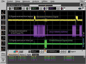
For this example mixed-signal application, we will explore an 802.11a wireless LAN access point as shown in Figure 1. Essentially, this system takes data from a wireless laptop, demodulates the signal down to baseband, and then converts the signal to a wireline signal onto a LAN.
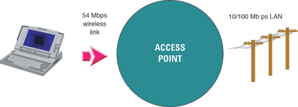
There are two main parts of this design that communicate through a PCMCIA interface. From the antenna of the access point, there is an RF processor that demodulates the transmitted signal to a baseband processor. From there, the baseband processor decodes the OFDM (orthogonal frequency domain modulation) signal and sends the data to an embedded system that then sends the data out to the LAN.
This mixed-signal system contains a 32-bit PowerPC embedded processor with a 100 MHz SDRAM and a simple LAN controller bus that communicates with the processor to send data out to the network.
The access point is a fairly small device, with two PC boards folded on top of one another. Figure 2 shows how the boards look when they are unfolded. The entire system is bidirectional, but in this example we will look at a transmission from the computer to the network.
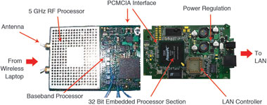
This example application is a classic mixed-signal system. There are analog, digital and embedded processor and DSP components, and the MSO is the perfect tool for looking at mixed-signal types and speeds from these elements simultaneously.
Viewing analog and digital signals simultaneously
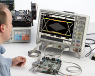
Figure 3 shows the MSO probe connections to the analog and digital signals of an access point PC board. For our demonstration, we connected the access point to a LAN, where it then sent information to a laptop PC with a wireless LAN card installed.
We executed a refresh command of the laptop’s Web browser and captured the resulting packet of information on the MSO.
The signals being measured by the analog channels of the MSO are the output of the baseband processor, the Ethernet signal out, and one data bit of the fast SDRAM bus. In this example, the SDRAM has edge speeds of up to 1 nanosecond. This edge speed requires an oscilloscope with a 1 GHz bandwidth to accurately measure and display the signals.
The signals measured by the MSO’s digital channels include one direction of a full-duplex 4-bit bus that runs between the PowerPC and the LAN controller and also a clock signal. There are 16 digital channels available on the MSO, but for this application, we chose to view only five of the digital channels.
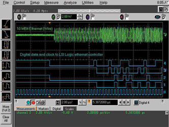
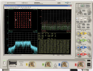
Figure 4 shows an acquisition of a single packet of information being sent through the access point as described above. The baseband, Ethernet and SDRAM signals are acquired on three of the MSO’s analog channels while the LAN controller bus signals, shown in blue, are acquired on the digital channels.
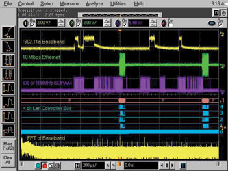
The red trace between the analog signals and the blue digital signals is a digital bus or a collection of digital channels presented as one waveform on the display. A 2 Mpts FFT computation of the baseband signal can also be seen at the bottom of the MSO display. These signals were all acquired in one acquisition on one instrument and screen.
Finding a debug method to capture and analyse all of this data on one acquisition has traditionally been a headache for most designers. Normally one would have to get the device under test into the same state to measure all of the signals, then move probes around, trigger multiple times, store waveforms on the display, and then find a way to correlate all this activity.
An MSO allows you to capture, display and measure all of this information simultaneously. It is easy to use and has all the functionality of a DSO, but has added digital channels and triggering capabilities. It simplifies the debug process by allowing you to see more channels and more time at once.
An MSO replaces today’s DSOs, and as can be seen from the screen in Figure 4, an MSO is the perfect tool for easily and efficiently analysing mixed-signal applications. In addition, the displayed waveform is enhanced with the scope’s 256-level intensity graded display to give a third dimension perspective to the waveform. This allows easy detection of anomalies and glitches.
Isolating the right information
In this example, there could be a packet error in the transmitted signal, so you may want to isolate a packet to see the interactions occurring in the system. On the wired Ethernet line is a sync burst that indicates the start of the transmission onto the LAN.
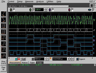
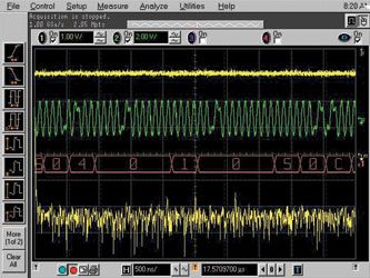
A 1010 pattern on the data lines of the LAN controller held for a duration of 5 microseconds generates this sync burst at the beginning of every 10 Mbit LAN packet. To isolate this condition, we set the MSO to trigger on the 1010 pattern for a duration of 5 microseconds. Figure 5 displays the 1010 pattern on D1 through D4 of the MSO’s digital channels, with DO assigned to the clock.
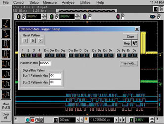
Because an MSO9104A has 16 digital timing channels and four analog channels, one can use the digital channels to perform a pattern trigger for a duration of time in order to trigger on a condition, such as a start of packet in this case. In fact, one can trigger across all 20 of the MSO’s channels. The digital channels can be set up quickly and easily using the trigger setup dialog box, as shown in Figure 6.
These extra digital channels allow the user to assign the four analog channels to analyse and measure the other signals of interest in the system. With an ordinary 4-channel DSO, four channels would be used just to generate a trigger, and there would be no channels left for debugging.
Although it is not shown in this example, you could set up a trigger condition based on the states of the four digital bits. You could also include the clock line and any of the analog signals in the trigger specification to narrow in on a problem.
With the Infiniium 8000 Series of MSOs, you can trigger on patterns that are up to 20 channels wide. This is impossible to do with a conventional DSO.
Using bus mode to gain visibility and insight
In Figure 5, the characteristics of the Ethernet signal change at about 1,5 divisions from the right side of the display. This is where the sync burst ends and the real data packet begins. To make it easier to identify the start of packet condition or any other condition of interest, you can configure the display of the digital channels to be in a bus mode to easily identify a digital pattern.
Figure 7 displays a bus representing eight digital channels. This screen shows the data coming across the bus as a hex display that is correlated with the Ethernet signal in the system. In this example, the 1010 digital pattern would be identified as 5 hex on the display, allowing you to easily and quickly identify the condition you are searching for.
You can display one or two 8-bit buses and each bus can have from 2 to 16 channels associated with it. You also can display any given digital channel individually, regardless of whether it is already part of one or both buses. The 16 digital timing channels give you not only added triggering capabilities, but also more visibility into what is going on in your design with this easy-to-use bus mode.
With previous debugging solutions, correlating triggers and signals has been difficult and time consuming. Designers needed to use multiple instruments to set up a trigger and then find a way to time correlate the instruments. An MSO makes triggering and signal correlation easy. Many designers prefer to use an MSO for debugging their mixed-signal designs because of the viewing capabilities such as bus mode and the ability to trigger across 20 channels.
Capturing long time periods
Why is deep memory important for debugging mixed-signal designs? Because it lets you achieve long capture time and high resolution. In this example, you need deep memory to capture a long period of time with high resolution because of the range of signal speeds. Without deep memory, you can achieve either long capture time or high resolution, but not both simultaneously.
The sample rate of an oscilloscope changes as you slow down the timebase or sweep speed. The scope must reduce its sample rate as the sweep speed is slowed down in order to capture enough time to fill the entire display without running out of memory. Keeping the sample rate as high as possible is critical, because it ensures that you are capturing your signals at full resolution, eliminating aliasing and measurement errors.
Often when debugging a complex system, you do not know exactly what the problem is, so you cannot set up the scope to trigger on it. You have to trigger on something more basic, such as an edge, and then look at the captured data to find the problem. This usually requires capturing a long span of time and then zooming in and out on the display, so again long time capture and high resolution are critical.
Perhaps most common is the need to correlate high-speed signals, which are often digital, with slower speed ones. In order to measure them both correctly with one acquisition, you need a time span that is long enough to show one or more full periods of the slower signals, and you need the sample resolution to be high enough to show full detail on the fast signals. Deep memory is essential for this ability.
In this example, you can acquire an entire packet of the data in about 500 microseconds of time. At a sweep speed of 200 microseconds per division, you need a minimum of 1 MByte of memory to view this packet of information with the sample rate set to 2 GSps. You need 1 MByte of memory just to capture the most basic transaction. If there are any errors or other transaction complexities, you would need even more memory.
The importance of deep memory in this application is shown in Figures 8 and 9. Figure 8 shows an acquisition of the faster SDRAM signal and the slower baseband signal. If you look at the fast SDRAM signal on the purple trace in Figure 9, you will see the same acquisition zoomed in by a factor of 200 000 times. Note that the rise time is about 1,5 nanoseconds and the time scale is 2 nanoseconds per division.
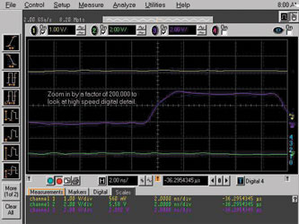
In this measurement, the scope is stopped and this analysis is performed on the single original acquisition. Without deep memory sustaining the high sample rate, there would not be nearly enough underlying data to support this amount of zooming.
The MSO’s MegaZoom deep memory automatically adjusts the memory depth so that as you change the time per division, the scope always samples with the maximum sample rate and memory depth available.
Also, MSOs come standard with 8 Mpts of deep memory per channel that allows you to capture slower signals and still see the details on fast signals all in one acquisition. The MSO automatically keeps the sample rate at its maximum setting based on the memory depth so that you can see the big picture and then zoom in on the details without having to trigger twice.
Traditionally, deep-memory scopes have had slow update rates, and they respond sluggishly to user inputs. This is not true for MSOs with MegaZoom deep memory. This memory responds instantly to changes, even with the deepest records, up to 128 Mpts.
This instant response is enabled by a custom architecture that captures data into acquisition memory and rapidly post-processes the data in the hardware for display and measurements. This architecture makes it possible to provide the waveform update rate and front panel responsiveness you need to get your job done more easily.
In order to make the 1,5 nanosecond measurement accurately, a high-fidelity active probe such as the Agilent 1156A is needed. This probe features very low input capacitance and properly damped tip resistance to enable it to make very unobtrusive and high-fidelity measurements.
Frequency domain measurements and analysis
Looking at the baseband signal in Figure 10, we see the time view along with bit 0 of the SDRAM bus. Because this comes from the wireless signal, it is valuable to also look at it in the frequency domain. You can make FFT measurements with an MSO, just like you can with a DSO.
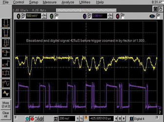
Figure 11 shows the FFT of the baseband signal. The MSO performs an FFT of all the data on the screen. This allows you to zoom in and out on the portion of the time record that has the frequency content of interest. It also makes it easy to compare the spectral content of different regions of the time-domain signal. In this case, most of the energy is located in the leftmost division of the FFT. You can see how the energy spans a broad, relatively even frequency range.
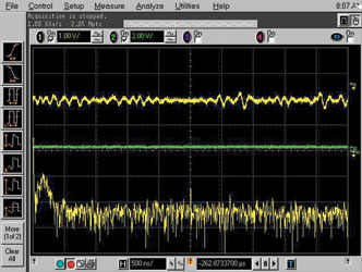
Figure 12 shows the beginning of the baseband transmission. In the first horizontal division of the FFT, instead of a broad, somewhat uniform distribution of frequency content, there are some distinct spectral lines. These lines indicate that the beginning of the baseband packet has a sync period just as the wireline side does. However, it is easier to see this event in the frequency domain.
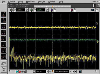
There are also some noise spikes on the FFT in Figure 12. These spikes could be caused by an unintended coupling in the system. In this access point, there is a high-power line driver on the wireline side in close proximity to a sensitive RF receiver on the wireless side that may be causing a coupling problem.
Modulation domain measurements and analysis
Figure 13 shows the WLAN IF signal being demodulated. When the Infiniium oscilloscope is combined with the 89601A VSA software, the scope can be used as a modulation domain analyser. BBIQ can be captured with any of the Agilent MSOs along with IF and RF if within the oscilloscope bandwidth.
Time correlate analog, digital and spectral information
Using the MSO’s digital channels can provide more detailed insight into the possibility of coupling. Figure 14 shows the digital bus turned back on and the time delay moved back to very near the original trigger point. In the live display and debug of this application, moving the horizontal delay back and forth showed that the noise spikes on the FFT measurement changed in magnitude based on which data was present on the LAN signal shown by the hex readouts of the bus mode.
The next step in the analysis would be to identify the data sequence that correlates to the highest levels of noise on the FFT display and further analyse that condition. For example, you could alter the PowerPC programming to repeatedly send out the corresponding data sequence attributed to the noise spikes.
From there, you would then look more carefully at the FFT with a spectrum analyser to determine the root causes of the coupling.
| Tel: | +27 12 678 9200 |
| Email: | info@concilium.co.za |
| www: | www.concilium.co.za |
| Articles: | More information and articles about Concilium Technologies |


© Technews Publishing (Pty) Ltd | All Rights Reserved
 printer friendly version