


This article from Agilent Technologies explains the reality and the mathematics behind digital multimeter (DMM) resolution and DC noise specifications, which directly correlate to the number of digits available from the DMM at a given resolution and speed.
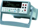
In this article, the 6½-digit Agilent 34410A DMM is used as an example.
DMM accuracy and resolution
Table 1 shows the DC voltage accuracy specifications for the 34410A DMM. On the 10 V range, and with the integration time set to 100 PLC (power line cycles - 1 PLC is 16,667 ms for countries using 60 Hz AC line frequencies), we see that the spec is plusmn;(0,0015% x reading + 0,0004% x range).
From Table 2, we also see that on the 10 V range, and for integration times of less than 100 PLC, we must add 0,0003% of range to the accuracy to account for DC noise errors.
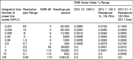
Suppose that we wanted to read a voltage that was previously calibrated, traceable to NIST standards, to be exactly 5 000 000 V and we wanted to measure this on the 10 V range at an PLC of 0,06 (1 ms). We would expect the accuracy to be ±(5,0 x 0,000015 + 10 x 0,000004 + 10 x 0,000003), or ±145 μV, and thus we would expect the DMM to display a steady reading somewhere between 4,999855 and 5,000145 volts, depending on how accurately we calibrated it. Since there is some unspecified base level of DC noise already included in the accuracy specification and we added 30 μV of additional noise to it, we would expect to see something over ±30 μV of variation in the readings due solely to DC noise. The peak-to-peak noise is thus something over 60 μV. As this article will show, this represents an rms noise of approximately 60 μV/6, or 10 μV. In fact, the DC noise specification is 15 μVrms on the 10 V range, so we would infer that 5 μVrms was the unspecified DC noise that had been included in the accuracy specification.
Analog-to-digital converter performance accounts for all DC noise errors. The second column in Table 2 shows the DC noise specifications for this DMM. Note that it varies in relation to the number of PLCs that are chosen. For example, if NPLC = 0,06 (0,001 second, or 1000 readings/s), the A/D converter in this DMM has an error of ±1,5 ppm rms x range. On the 10 V range, this is ±15 μmVrms.
Ultimately, we want to know how many digits of resolution we can get for a given integration time. Taking the 10 V range again as an example, we would expect to see a variation from reading to reading of ±15 μV. Suppose our DMM was calibrated such that it read exactly 5,000000. We would expect readings to range from 4,999985 to 5,000015 most of the time. It is plain that the 1 μV digit is useless in this case, so we would actually expect the readings to be displayed as 4,99998 to 5,00002.
This is a 6-digit reading. Since we are on the 10 V scale and this DMM has 20% overrange capability, readings up to ±12,00000 can be taken. The most significant digit can only go from 0 to 1, so it is called a digit. Thus, the DMM is said to be a 6 digit DMM at this reading rate, one in which the last (10 μV) digit can be expected to change from reading to reading by ±2 counts most of the time. ('Most of the time' means 68,3% of the time, which is the definition of rms.) In reality, the actual performance has been measured to be better than the spec, and we would normally see only a ±1 count change in the last digit 68,3% of the time.
The way we measure the DC noise performance is by applying a DC voltage and taking a few hundred sample readings. Since we also wish to eliminate any errors in a source, it is simplest to just short the input terminals (which gives us a 0 V input) and ignore nonlinearities that might cause some additional errors at higher input-voltage settings. We then get a distribution in the readings that follows a statistical model. If the samples were distributed equally, we would call it a uniform distribution.
Quantisation
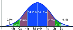
A classic paper on quantisation error written in 1948 by Bell Labs shows that the act of quantising an analog signal results in a uniform distribution, so if our measured readings were distributed in this way, we would say that the DMM readings were 'quantisation-limited.' In other words, the act of converting the analog value to digital would be the primary source of the error. If the samples were distributed in a Gaussian form (Figure 2), the noise would be said to be caused by 1/f noise, thermal noise, nonlinearities and other analog errors. The manner in which we would compute the rms value is different for the two cases.
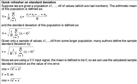
The Bell Labs paper on quantisation error shows us that the rms noise is given by:
rms noise = ideal resolution/√12
where ideal resolution = voltage span/2n (n = number of bits in the A/D)
For example, an 8-bit A/D that can measure voltages from -1 to +1 has an ideal resolution of (1 - (-1))/256 = 7,8 mV, and we would expect to measure an rms noise of 2,3 mV, not including any other analog errors due to circuitry between the input terminals and the A/D converter.
In most modern DMMs, the A/D converters have enough bits of native resolution that this quantisation error is much smaller than other errors and can be ignored.
Since the other sources of error are distributed in Gaussian form, we can use the formula for standard deviation to compute the rms value (see below).
Practical experiment
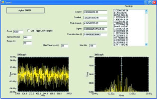
A Visual Studio.NET program was written to control a 34410A DMM using Agilent's T&M Toolkit software to make the graphing job and the instrument control easy.
The inputs were shorted and 1000 samples taken on the 10 V range with an aperture time of 1 ms. The data was plotted as raw data and as a histogram, as shown in Figure 3. Although quantisation 'buckets' are clearly visible in the graph on the right, the overall pattern is that of a Gaussian distribution. This DMM is therefore not quantisation-limited. In this case, 8,2 μVrms, or 45,5 μVp-p (±22,8 μV) of DC noise was measured. (Remember that the spec was 15 μVrms, so it is well within this limit.)
Thus, there is a 68,3% probability that the measured value will be within ±8,2 μV of the actual value. A peak-to-peak value can be called three things that all have the same meaning: ±3 sigma, six-sigma, or 99,7% probability. Thus there is a 99,7% probability that the measured value will be within ±22,8 μV of the measured value. Since these measurements were taken on the 10 V range, the reading would best be displayed as 0,00000, and we might expect to see it change from -0,00001 to +0,00001 once in a while and go as high as ±0,00002 on a less-frequent basis.
An effective number of digits (ENOD) can be calculated as follows:
ENOD = log10 (positiveSpan/rmsNoise) for a 68,3% probability (±1 sigma)
or
ENOD = log10 (totalSpan/ppNoise) for a 99,7% probability (±3 sigma)
Companies do not usually publish the internal span of their A/D converters, so it may not be possible to derive this number when you compare specs from one company to another. In the case of the 34410A, the internal range is ±14 V on the 10 V range, even though the usable range is artificially limited to ±12 V. So, plugging in,
ENOD = log10 (14/0,0000082) = 6,2 digits (68,3% probability)
or
ENOD = log10 (28/0,0000455) = 5,8 digits (99,7% probability)
Since the spec is based on rms noise, not peak-to-peak noise, we would call this a 6½ digit DMM on the 10 V range at 1000 readings/s. The same method can be used to calculate the ENOD for other ranges and speeds.
One can also use signal-to-noise + distortion ratio (SINAD) to calculate ENOD. There is a well-known formula relating signal, noise, harmonic distortion and effective number of bits in the A/D:
N (effective) = (S(N + D) - 1,8)/6,02
Where S/(N+D) is the ratio of the signal power of a full-scale input to the total power of noise plus distortion, expressed in dB. This formula reinforces the notion that noise errors come from many sources, not merely quantisation error. A full discussion of this method of measurement is beyond the scope of this article.
Conclusion
Establishing the number of usable digits for a DMM depends upon its calibrated accuracy and the performance of its A/D converter. In most modern DMMs, the quantisation error due to analog-to-digital conversion is far less than that of other analog errors and can be ignored. The effective number of digits is based on rms noise performance, which is a Gaussian distribution of noise that is generated inside the DMM by thermal noise, 1/f noise, harmonic distortion and other analog errors.
| Tel: | +27 12 678 9200 |
| Email: | [email protected] |
| www: | www.concilium.co.za |
| Articles: | More information and articles about Concilium Technologies |


© Technews Publishing (Pty) Ltd | All Rights Reserved
 printer friendly version