


Digital multimeters (DMM) are the workhorses of the electronics industry. Almost all of the electronic products we use in our personal and professional lives are built or serviced using multimeters.
Different DMM applications require different degrees of attention to specs. A technician checking a logic power supply can use his trusty bench DMM confidently to verify that the supply is within a few percent of 5 V. However, when the job requires testing critical circuits, checking precision components, making fine adjustments in production, verifying compliance with industry standards or taking measurements outside the controlled environment of the lab, the meter’s specifications need to be evaluated carefully.
A solid understanding of specifications is critical when one is evaluating the suitability of DMMs for an application, or when confidence is required that readings accurately reflect reality. This article discusses some of the background behind DMM specifications and spec sheets. It defines the various elements of DMM specs and gives tips on how to apply them.
Specifications and the spec sheet
Whenever a measurement is taken with any meter, a gamble is implicit, a gamble that the instrument is going to give the ‘real’ reading. Fortunately, it is a very safe bet that a quality multimeter will deliver readings that coincide with reality. Specifications quantify the confidence of getting accurate readings and the risk of seeing inaccurate readings.
A specifications document is a clearly written description of an instrument’s performance. It should quantify an instrument’s capabilities objectively under well defined operating conditions. From this formal definition one can draw the characteristics of good specifications:
* Completeness – any factor that impacts uncertainty is covered, including operating limits such as humidity, altitude or vibration.
* Clarity – all efforts should be made to make the specifications straightforward.
* Objectivity – does not attempt to mislead for the sake of promotion.
A well written specification should maintain the same level of integrity as a medical chart or bank statement. Manufacturers must stand firmly behind their specs and the user should fully expect that the information they are getting is accurate and complete. On the spec sheet should appear measurement uncertainty specs and modifiers that affect the uncertainty. One will also see operating limits that constrain the environment in which the uncertainty specifications will hold true. These are stated in numerical values (eg, humidity) or with reference to international standards (shock and vibration).
First let us take a closer look at how to quantify measurement uncertainty.
Where do uncertainty specifications come from?
The main job of a DMM specification is to establish the measurement uncertainty for any input in the instrument’s range. The spec answers the question, “How close is the value on the meter display likely to be to the actual input to the meter?” Meter manufacturers bet their reputations on how a large population of instruments is going to behave for the duration of calibration cycle (typically one year). Instrument engineers and metrologists use laboratory testing and carefully applied statistics to set the specs.
DMM specifications apply to a particular model (ie, design), not to any individual instrument. Any single instrument of a particular design should perform well within the specification, especially toward the beginning of its calibration cycle. A model’s specs are based on testing a significant sample of products and analysing the collected data from the instruments.
If one takes measurements of a nominal input from, say, 50 instruments of the same design, a range of readings will be obtained. Many of the instruments will have the same readings, but some variation would be expected due to normal uncertainty. For example, the readings from 50 Fluke Model xyz DMMs hooked up to the same precision calibrator outputting 10 V can be recorded. A narrow spread of readings around 10 V will be recorded. The mean (average) of all the measurements can be calculated, which should be 10 V. One can also calculate the standard deviation of the readings (Equation 1).
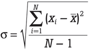
Equation 1 where N = sample size; X = measurement
The standard deviation is a measure of the ‘spread’ of the sample of measurements, outward from the mean. This measure of spread is the basis of uncertainty specifications. If a plot is made of the number of times each reading occurs, a bell-shaped normal distribution should result (almost all measurements follow a normal distribution, including those made with simple instruments like rulers and measuring cups). Figure 1 shows a normal distribution curve centred at 10 V.
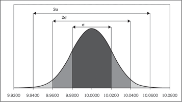
Using experimentation and experience, instrument designers set specifications by assuming a normal distribution and finding the standard deviation for a significant number of design samples. Adopting a normal distribution allows us to relate standard deviation to the percentage of readings that occur, by measuring the area under the curve – 68% of the readings will be within 1 standard deviation of the mean; 95% of the readings will fall within 2 standard deviations of the mean; 99,7% of the readings will fall within 3 standard deviations of the mean.
Statisticians refer to these percentages as confidence intervals. They might say, “We are 95% confident that a reading will not be more than 2 standard deviations of the actual value.” In the simple example above: 1 standard deviation corresponds to ±0,02 V; 2 standard deviations correspond to ±0,04 V; and 3 standard deviations correspond to ±0,06 V.
So the questions for the manufacturer become, “How many standard deviations do we use for our spec and what confidence interval do we use to build our specs?” The higher the number of standard deviations, the lower the probability that an instrument will fall out of spec between calibrations. The manufacturer’s internal engineering standards will determine how many standard deviations are used to set the spec. Fluke uses a confidence of 99%, which corresponds to 2,6 standard deviations on a normal distribution.
Traceability and specifications
So far it has been described how much uncertainty can be expected from a DMM, but it has not been discussed how to make sure everybody is talking about the same Volt, Ohm or Amp. DMMs must trace their measurement performance back to national laboratory standards.
DMMs are usually calibrated using multifunction calibrators like the Fluke 5700A or Fluke 9100. But there are usually a number of links between the DMM and national standards, including calibrators and transfer standards. As one moves through the chain between a DMM and the national standards lab, the calibration standards become increasingly accurate. Each calibration standard must be traceable to national standards through an unbroken chain of comparisons, all having stated uncertainties.
So the uncertainty of a DMM depends on the uncertainty of the calibrator used to calibrate it. Most DMM specs are written assuming two things:
* The DMM has been calibrated using a particular model of calibrator, usually specified in the DMM service manual.
* The calibrator was within its operating limits and traceable to national standards.
This allows a DMM manufacturer to include the uncertainty of the calibrator in the DMM uncertainty specs. If an uncertainty is listed as ‘relative’ this means the uncertainty in the calibrator output has not been considered and it must be added to the DMM uncertainty.
Elements of digital multimeter specifications
Among the many standards that govern instrumentation, there is no standard for writing DMM specs. Over the years, though, manufacturers have converged on similar formats, making it a bit easier to compare multimeters. This article covers the most common conventions for specifications. As described above, uncertainty specifications define a range around a nominal value. When taking a measurement within the specified limits of time, temperature, humidity, etc, the user can be confident that they will not get a reading outside that range.
Time and temperature are crucial for determining uncertainty. Electronic components experience small changes or ‘drift’ over time. Because of this, DMM uncertainties are valid only for a specified period of time. This period usually coincides with the recommended calibration cycle and is typically one year. At calibration, the clock starts over again and the uncertainties are valid for another period.
Temperature affects the performance of every component in an instrument—from the simplest resistor to the most elegant integrated circuit. DMM designers are good at building circuits that compensate for temperature variation. This ability to operate at various temperatures is captured in a specified operating range and is often accompanied by a temperature coefficient (more on this later).
Multimeter uncertainties cannot be given as simple percentages, although it is tempting to over simplify. One might see a sales brochure that touts 'basic accuracy to 0,002%'. This is only giving a small part of the picture, and it is usually an optimistic view of the data. The reasons for complexity in the specifications have to do with the multimeter’s ability to perform many different measurements, over many different ranges, using several different internal signal paths.
Consider the diagram in Figure 3. It shows the analog signal path for a DC voltage measurement, also known as the ‘front end’. Each block contributes uncertainty in the form of nonlinearity, offset, noise and thermal effects. The front end contributes most of the uncertainty of the instrument. Depending on the design, changing ranges affects the divider performance or the amplifier performance or both. Internal noise, for example, has a greater relative impact on lower ranges and at the low ends of ranges.
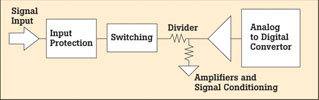
Changing functions alters the signal path. For example, a resistance measurement requires the addition of a current source to the analog path. So each function and range must be specified in a way that considers the effects of non-linearities, offsets, noise and thermal effects. Table 1 shows the elements of a DMM specification and gives examples for each.
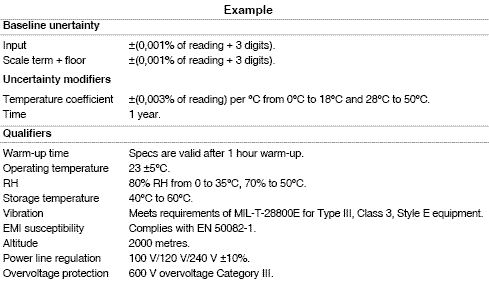
Baseline uncertainty specifications
Baseline specifications are usually given as ±(percent of reading + number of digits) or ±(percent of reading + number of counts). ‘Digits’ or ‘counts’ are used interchangeably and they indicate the value of the least significant digits for a particular range. They represent the resolution of the DMM for that range.
If the range is 40,0000 then one digit, one count, is worth 0,0001.
Let us say one wants to measure 10 V on a 20 V range in which the least significant digit represents 0,0001 V. If the uncertainty for the 20 V range is given as ±(0,003% + 2 counts) the uncertainty can be calculated in measurement units as ±(0,003% x 10 V + 2 x 0,0001 V) = ±(0,0003 V + 0,0002 V) = ±(0,0005 V) or ±0,5 mV.
Some spec sheets use the form: ±(percent of reading + percent of range). In this case one simply multiplies the maximum reading for the range by a percentage to get the second term. In both cases the second term is called the ‘floor’. The floor considers the effects of offsets and noise associated with a single range as well as those common to all ranges. Ignoring this term can have significant consequences, especially for measurements near the bottom of a range.
Uncertainty modifiers
Modifiers can be applied to the uncertainty specs to account for common environmental or time factors. Some specifications will give not only one-year specs, but also specs that apply for, say, 90 days after calibration. The 90-day spec will be tighter than the 1-year spec. This allows a DMM to be used in more demanding applications by calibrating more frequently.
For reasons already covered, uncertainty specs are valid over a specified temperature range. Commonly the range encompasses ‘room temperature’, from 18°C to 28°C when calibrated at 23°C. Over a wider range the uncertainty can be modified to account for the temperature.
Say one needed to take the same 10 V measurement performed above, at a field location where the temperature is 41°C. The temperature coefficient of the DMM is given as: ±(0,001% of reading) per °C from 0°C to 18°C and 28°C to 50°C. The temperature is 13°C above the 28°C boundary for using unmodified baseline uncertainty. For each degree above the boundary, we have to add 0,001% x 10 V = 0,1 mV/°C to the baseline uncertainty. The added uncertainty at 41°C is therefore 13°C x 0,1 mV/°C = 1,3 mV. So the total voltage uncertainty, combining the baseline uncertainty calculated in the example above and the temperature modifier would be ±(0,5 mV + 1,3 mV) = ±1,8 mV. Notice that the modified uncertainty is more than three times larger than the baseline.
Qualifier specifications
DMM uncertainties depend on other conditions besides time and temperature. Environmental factors such as storage temperature, humidity, air density and electromagnetic radiation can affect uncertainty. The DMM must receive reasonably clean power if its precision internal power supplies are to function properly.
Some qualifiers can be easily specified by numerical values, like power line regulation, altitude and relative humidity. DMMs are not hermetically sealed, so air becomes a component of their circuitry. The electrical characteristics of air are affected by density (altitude) and humidity, so designers set boundaries on these parameters. Excessive storage temperatures can irreversibly alter the operating characteristics of electronic components.
More complex qualifiers like over-voltage protection, shock and vibration, or electromagnetic compatibility are given by noting compliance with standard measurement techniques and limits. International standards documents for these characteristics typically require a series of test procedures along with applicable limits. Adding all of the limits would render the DMM specifications too cumbersome, so DMM designers just list the standards with which the DMM complies.
Comparing different digital multimeters
When one is evaluating the suitability of several digital multimeters, the best approach is to choose a set of measurements and conditions that approximate your application. First, make sure the qualifiers of each DMM are compatible with the application environment. Then consider all of the functions (DC volts, AC volts, DC amps, ohms and so forth) and ranges are likely to be used. If a lot of measurements near the bottoms of ranges are going to be made, then comparisons with low readings should be made to check the contribution of the floor. For each measurement, the uncertainty should be converted into measurement units like Volts, Ohms or Amps. The uncertainties should be compared in measurement units to decide which DMM is better suited to the task at hand.
The ability to work with DMM uncertainty specifications is a fundamental engineering skill. When two different answers are obtained from two different DMMs, measurement uncertainty might explain the difference. When the performance of DMMs needs to be compared to decide the right tool for the job, being proficient with uncertainty specs will help the user compare apples to apples. And whenever one depends on an important measurement, they can be comfortable understanding how well their instrument will really perform.
| Tel: | +27 10 595 1821 |
| Email: | [email protected] |
| www: | www.comtest.co.za |
| Articles: | More information and articles about Comtest |


© Technews Publishing (Pty) Ltd | All Rights Reserved
 printer friendly version