


Most engineers will be able to get through an entire career without having to think about the mathematical realities that underlie the principles of randomness and entropy, even though many use or design applications that rely on them to ensure the security of their interactions.
For the most part, engineers simply take the vendor’s specifications at face value when incorporating the cryptography hardware (and the code that supports it) into designs. Unfortunately, some recent discoveries about the more subtle and not-well-documented characteristics of random noise sources have shown that you may not be getting all the security you paid for.
One of the best examples of this phenomenon is the humble ring oscillator, whose phase jitter is commonly used as the primary ingredient for the seed sequence used to prime the pseudo-random number generators frequently found in secure networking gear and more specialised military communications equipment.
While it was generally believed that the oscillator’s phase variations are deeply unpredictable from moment to moment, a closer look reveals that much of its short-term activity can be mathematically categorised and, therefore, predicted.
Fortunately, this deeper understanding of the ring oscillator’s behaviour also reveals the conditions under which it can be properly used to produce seeds that embody sufficient randomness (entropy) to provide the true 256-bit security required to keep communications beyond the reach of a massive cyber-attack.
This article is not intended to make readers an expert on the fine points of random number theory or the deep math that accompanies it. Its more modest aim is to familiarise you with the concepts needed to use ring oscillator-based noise sources properly.
Equally important, you will learn how to instantiate a practical seed generator in low-cost FPGA technology and some simple techniques to verify the actual level of entropy (security) a design will produce for a particular application. If you are new to all this, a quick primer on entropy and security is provided below. If you are a seasoned security pro, feel free to skip ahead to the next section.
Entropy and security
Virtually every form of secure communication relies on a random number generator to protect its users from the prying eyes of hackers, unfriendly governments, industrial spies and other unwelcome intruders.
In these systems, random numbers are used to produce the secure keys for encrypting and decrypting data and commands. Besides securing commercial, government and military networks, these advanced encryption techniques are playing a critical role in the ‘Internet of Things’ where networks of so-called Smart Objects autonomously manage buildings, industrial processes and even entire power grids.
Randomly generated numbers are also used to produce NONCEs (numbers used once) that are essential to thwarting replay attacks in Mil-TAC radios, secure routers, IFF systems, missile launch controls and C3 products, not to mention ensuring that casinos and online gaming systems deliver the odds they are programmed for.
In nearly all these applications, a pseudo-random number generator (PRNG) actually produces the high-speed streams of random digits required to support hundreds, and sometimes even thousands, of secure transactions per second.
Since a PRNG’s logic is deterministic, a skilled hacker who knows its internal state for a given output can use the generator’s relatively low ‘forward resistance’ to successfully predict its subsequent outputs. This means that the security of the PRNG’s output is highly dependent on the absolute unpredictability, also known as entropy, of the seed number it is fed.
If the seed number has some level of predictability, it is possible to observe the encrypted data stream and make highly educated guesses about some of the variables used to seed the PRNG. A low level of entropy in the seed for a 256-bit SSL key can reduce its number of unknown bits to 80 bits or less, making it vulnerable to a brute force attack.
Perhaps the best example of this vulnerability is the Secure Socket Layer (SSL) encryption protocol used by early versions of the Netscape browser in the mid-1990s. At the time, Netscape’s implementation of the protocol was based on pseudo-random variables derived from a PRNG that used the time of day, the host computer’s process ID, and the parent process ID as seed values, all of which could be inferred by various means.
Similar problems have been identified (and fixed) in other software, including several variants of Linux and at least one earlier version of the MS Windows operating system.
The key to preventing such attacks is to keep the PRNG regularly seeded with a random number that has a high degree of entropy, usually from some sort of physical phenomenon not related to the equipment using it.
Many different types of seed sources, including lava lamps (see Figure 1), have been used with varying degrees of success but most systems employ a hardware random number generator (RNG) based on phenomena that generate a low-level, statistically random noise signal, such as thermal noise, the photoelectric effect or other quantum-level behaviours.

One of the most commonly-used hardware RNG schemes generates its values based on the relative phase difference between a stable frequency source such as a quartz crystal oscillator (XO) and a less stable frequency source, typically a ring oscillator (RO).
Constructed using an odd number of inverters connected in a circular string, the resulting unstable logic state ripples through the oscillator at a frequency determined by the circuit’s cumulative propagation delays. The ring oscillator’s inherently high level of phase noise makes it a poor choice for many applications but becomes a useful feature for RNG applications.
The time difference between the edge of a stable frequency source and the ring oscillator’s signal can be captured and used to produce a random bit. The RNG’s seed value is built up by producing a series of random bits with a delay of 1000 or more cycles between readings to ensure the ring oscillator has drifted sufficiently to give a high level of entropy.
The truth about ring oscillators
Ring oscillators were assumed to be relatively good entropy sources because it was believed that they produced a random walk in phase where, for every transition, the deviations in its flipping time was uncorrelated and independent (‘white’ in frequency).
This was discovered to be not quite true when a deeper analysis of the ring oscillator’s phase noise was conducted as part of the research related to developing secure IP for Microsemi’s programmable logic products.
The study was undertaken to characterise the ring oscillator’s noise process, with the intention of finding answers to several fundamental questions, including the following:
* What is the optimal time to wait before sampling the ring oscillator’s state?
* How does the variation in phase increase with time?
* What mathematical models best describe the random process?
* What physical processes are responsible for the oscillator behaviour?
Perhaps the most important issue was to take a closer look at the commonly held assumption among cryptologists that ring oscillator 'flipping times [are] independent and identically distributed'.1 If this were true, the oscillator would display a ‘random walk in phase’ characteristic.
It was suspected that this assumption is not accurate because it has been observed that the frequency of ring oscillators drifts widely over time. This observed behaviour does not match the theoretical behaviour of the random walk model commonly used to describe ring oscillator phase noise.
Traditional methods for measuring phase variation in the time domain are based on the concept of standard variance - the difference between the sample and the mean (or squared deviation from mean), as illustrated in Equation 1.
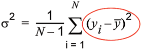
The bar over the y term in Equation 1, and subsequent equations, means the average value. The y² term is circled here to highlight the fact that it is hard to estimate accurately in the presence of higher-order terms. This means that the introduction of higher-order drift terms reduces confidence in the estimate of the mean, especially over longer measurement intervals.
It follows that confidence in the estimate of the standard variance also degrades in the presence of long-term drift. The standard deviation (σ) is the square root of the standard variance (σ²).
Beware entropy inflation
While useful for many applications, this mathematical technique has a blind spot for certain types of behaviour. Specifically, it cannot distinguish between real changes in the phase it sees and other higher-order noise terms, such as a random walk in frequency, or linear frequency drift.
As a result, the equation becomes divergent if, over longer averaging intervals, these higher-order terms cause the mean to wander.
For example, if we compute the standard variance of an oscillator whose frequency varies widely, the result grows progressively larger as the averaging intervals we use grow longer, despite the fact that the phase variations produced by the oscillator remain constant.
The resulting inaccuracies in the mean can produce entropy inflation – a computed variance much higher than the actual variance when measured for long sample periods.
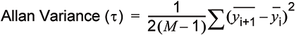
A mathematical tool known as the Allan Variance deals with standard variance’s bias problem by adding a function that compensates for some of the most common elements that cause long-term drift.
As shown in Equation 2, the technique uses the difference between adjacent values of the average value calculated over a given sample period (τ0), where M is the total number of fractional (normalised) frequency samples. Comparing each sample against nearby values produces a ‘back difference’ that reduces the errors induced by the mean drifting over time.
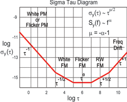
Using Allan Variance, τ can be swept over incrementally longer sampling periods (microseconds to hours), and the results can be used to produce a variance curve (sigma-tau log-log plot), as shown in Figure 2. Adjacent sample periods can be overlapped in time to reduce analysis noise; that is, improve the confidence interval.
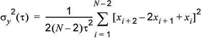
A more computationally efficient way to compute the Allen Variance is shown in Equation 3. Instead of averaging the frequency samples over the measurement interval (as in Equation 2), it uses the starting, middle and end phase samples to provide an identical result.
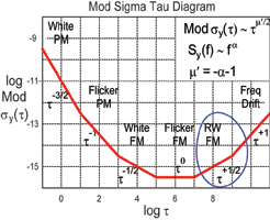
Modified versions of the Allan Variance can be used to extract other higher-order effects beyond simple frequency variation. For example, the modified Allan Variance used to produce the Sigma-Tau plot shown in Figure 3 employs additional averaging techniques that allow it to distinguish between white PM and flicker PM. The different slopes of the Sigma-Tau plot provide graphic evidence of the different types of noise processes at work.
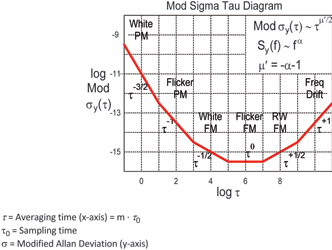
A Time-Dorman Power Law slope using a modified Allan Variance technique can distinguish between second- and third-order phase effects such as white- and flicker-phase modulation.
The results of the Allan Variance analysis and its related methods raise concerns that if the behaviour of ring oscillators had been characterised using simple standard deviation techniques, much of the short-term behaviour that had been assumed to be highly random phase noise is actually a random walk in frequency and other phenomena that are more predictable over short time intervals.
While a random walk in frequency produces a great deal of entropy (randomness) over long time periods, its short-term behaviour is much more predictable (has a lower level of entropy) than a random walk in phase. This raises the concern that if the RO’s behaviour is dominated by frequency-related phenomena, the seed numbers produced by ring oscillators could contain significantly less entropy (less unpredictability) than previously understood.
Under certain conditions, these reduced entropy values could constitute a potentially serious security weakness. For example, an encryption system using an RO-based entropy source might be delivering seeds whose reduced entropy levels made it possible to correlate the state of a significant number of bits in the key to other nearby bits.
If the entropy level was sufficiently low, the subsequent bit stream could enable an attacker to make educated guesses about the PRNG’s internal state. This would eventually reduce the uncertainty in the keys it produced to the point where its associated system was vulnerable to a brute force attack.
Looking at phase noise in the time domain
To explore this theory, an experiment using time domain techniques was developed. Time domain analysis was chosen because it is simpler and less complex than traditional frequency domain methods.
The capabilities of traditional frequency domain equipment are hard pressed when they attempt to separate phenomena of interest such as amplitude noise from phase noise. In addition, the longer sampling times (in some cases, 20 minutes or more) used by time domain techniques allows easier, more reliable analysis than attempting to use a spectrum analyser to measure low-frequency phase modulation so close to the carrier frequency.
Instead of the expensive equipment and complex test circuits used in frequency domain analysis, a test circuit and a simple time domain analysis tool was constructed using Microsemi’s SmartFusion customisable system-on-chip (cSoC) ICs (Figure 4).
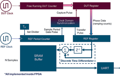
A cSoC, by definition, includes both a configurable FPGA fabric and a microcontroller. The one-chip test rig was configured to implement a 21-stage ring oscillator (RO) as a device under test (DUT). Other elements within the FPGA portion were used to construct an oscillator that could be used to program a gating window (consisting of m oscillator cycles).
Other FPGA logic was used to measure the phase state at the edge of each gate interval with respect to an external crystal oscillator (XO) reference clock (REF). A discrete-time differentiator compares the phase differences between the REF and DUT oscillators and stores the result in a block of the cSoC’s SRAM buffer.
A simple program was developed to run on the cSoC’s integrated ARM Cortex-M3 processor core that would collect the phase data from the SRAM and make it available for analysis by a PC or other computer via a serial UART channel.
Interpreting RO test data
With a means of reliably observing the RO’s behaviour in sight, it is time to consider how to interpret the data collected. If the commonly held assumption that the RO’s switching times are ‘independent and uncorrelated’ were true, a time domain waveform of its frequency samples would follow a Gaussian distribution and closely resemble a frequency domain plot of white noise.
In this case, integrating the frequency samples to produce a waveform of the RO’s phase behaviour would produce a time domain plot that looked like a random walk. For those unfamiliar with the concept, random walk behaviour is defined as when the standard deviation (σ) of an ensemble (a collection of test runs) grows as the square root of the averaging time (τ).
So, if the RO’s phase variations occur as a random walk, a power law (log-log) plot of their behaviour would resemble the Sigma-Tau plot shown earlier in Figure 3, displaying a slope of –1/2.
If, however, suspicions are justified that the RO’s phase deviation consists mostly of samples that have a higher order of correlation (are more predictable), they would produce a more positive slope when placed on a Sigma Tau plot.
The power law plot shown in Figure 5 represents the deviation of frequency samples collected from several time domain series and plotted using a Modified Hadamard Deviation (an improved version of the Allan Variation formula that compensates for higher-order effects).
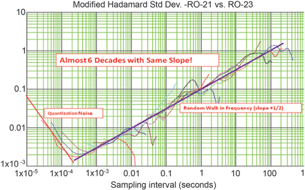
Most of the activity shows the Hadamard Deviation rising one decade for every two-decade increase in the sampling interval (a slope of +1/2). The exception to this trend occurs in the lower left hand corner of the plot, where the deviation reverts to a sharp negative slope as the sample interval drops below 1 ms, a sure indicator that quantisation noise is dominant in this region.
This leads to the conclusion that, for sample periods below 1 ms, the behaviour is more periodic and not truly random, making samples collected over short intervals completely unsuitable as an entropy source. For the sample intervals above 1 ms, the actual random jitter contained in the RO’s waveform begins to accumulate.
The linear slope produced for sample intervals above 1 ms is a signature characteristic of a random walk in frequency and not the random walk in phase that had been previously assumed. The linear power law behaviour exhibited across nearly six decades of sampling intervals is due to the fact that the noise added at each switching interval displays Brownian characteristics.
When these variations are integrated over time, they produce a cumulative phase error that looks like white noise which has been integrated twice (once even before it was measured). In other words, the noise displays a random run in phase, otherwise known as a random walk in frequency.
This underscores that the major component of the RO’s deviations are in frequency which varies as a random walk, causing its phase to vary as a random run, and therefore to be relatively predictable over short periods of time.
Since the truly random phase component of the deviation is a much smaller part of the signal’s behaviour than originally believed, a much longer time interval between samples (relative to the oscillator’s frequency) is required to produce phase relationships that contain a sufficient level of entropy.
Practical implications
The results of this experiment call into question several commonly held assumptions about the behaviour of ring oscillator-based entropy sources. Some of the more important findings include the following:
* The common perception that ring oscillator ‘flipping times [are] independent and identically distributed,’ appears to be wrong.
* The circuit’s flipping time noise appears to be dominated by Brownian (1/f³) circuit noise over a very wide range of frequencies. Brownian noise is random walk noise.
* The flipping time noise is integrated (again) when accumulated into phase behaviour, so it becomes a random run in phase or, equivalently, a power law characteristic of a random walk in frequency.
* Any assumptions about the ‘independence’ or ‘memory-less’ characteristics of oscillator noise should be carefully validated with experimental data before they are applied to any mission-critical design.
While many of these findings are primarily of interest to security theorists, the work also uncovered several items that are of critical importance to nearly any designer involved with security-oriented applications. On a practical level, designers working with high-security equipment must keep in mind that the amount of entropy available from RO-based PRNG seed generators may be much lower than common practice had suggested until now.
The experiment shows that, for the ring oscillator tested, using sample intervals of 1 ms or less produced deviations that were dominated by quantisation noise and contained virtually no entropy. For periods of 1 ms to 100 ms, the circuit produced increasing amounts of entropy as the sampling interval grew, but their magnitude was smaller than previously understood.
For the circuit we tested, at best, (assuming ideal conditions and that all bits have full entropy) we can expect about 1000 bits/s of entropy, allowing it to generate a maximum of roughly four 256-bit seeds per second. In reality, the oscillator will have other correlatable phenomena which reduce the actual entropy levels available to a PRNG.
Sampling periods of slightly longer than 1 ms are probably safe, as long as only one bit of entropy is extracted per sample. And, at these relatively rapid sample rates, each new design (or design modification) must be subjected to rigorous statistical tests (such as autocorrelation) to assure the extracted bits are truly uncorrelated.
It is expected that the phase variation behaviour of other ring oscillators will vary greatly, depending in large part on such variables as their operating frequency, the semiconductor process the circuit was fabricated in, and the characteristics of the circuit they are driving.
Although the magnitudes of the entropy levels they produce may vary greatly, it is likely that the general properties they display will be very similar to the one tested in this experiment.
The true entropy levels available from RO-based sources is still being studied and the effects not yet well understood enough to produce any additional engineering guidelines or rules of thumb that can be cleanly translated into design practices.
Despite this, the study has produced several ideas that should prove helpful in designing equipment which actually delivers the level of security intended:
* Analysis of your entropy source using time domain methods such as the Allan Variance technique is essential. Time domain techniques provide a simple, cost-effective way to characterise the physical circuit.
* Time domain analysis also makes it relatively easy to identify the different effects at play in the noise process and which process is dominant over each range of time intervals.
* If your design requires production of seed values at a sample frequency which produces insufficient entropy, consider using multiple ROs run in a parallel manner. A multiple-RO architecture has the added advantage of being harder to spoof through signal injection techniques.
* Characterising an entropy source using time domain methodologies such as the one described in this article is a reliable and cost-effective method of ensuring the security of existing products as well as new designs.
References
1. 'On the Security of Oscillator-Based Random Number Generators', Mathieu Baudet, et al.
Recommended reading: 'Handbook of Frequency Stability Analysis, W.J. Riley.' NIST Special Publication 1065; http://tf.nist.gov/general/pdf/2220.pdf
For more information visit www.microsemi.com


© Technews Publishing (Pty) Ltd | All Rights Reserved
 printer friendly version