


Controller area network (CAN) offers robust communication between multiple network locations, supporting a variety of data rates and distances. Featuring data-link layer arbitration, synchronisation and error handling, CAN is widely used in industrial, instrumentation and automotive applications.
Standardised under ISO 11898, with distributed multi-master differential signalling and built-in fault handling, various protocols such as DeviceNet and CANopen define implementations for physical and data-link layers. This article describes how to optimise settings for a given application, considering hardware restrictions such as controller architecture, clocks, transceivers and logic-interface isolation. It addresses network configuration – both data rate and cable length – explaining when reconfiguration of CAN nodes is necessary and how nodes can be optimally configured from the beginning.
Isolating the logic interface
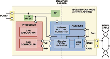
For harsh industrial and automotive environments, system robustness can be further enhanced by isolating the logic interface to the CAN transceiver, allowing large potential differences between ground nodes and providing immunity to high-voltage transients. An isolated CAN node can be formed by integrating a CAN transceiver with digital isolators. The ADM3052, ADM3053 and ADM3054 isolated CAN transceivers provide various options for powering the interface.
For DeviceNet networks, the isolated side can be powered from the bus, so the ADM3052 integrates a linear regulator to provide a 5 V supply from the 24 V bus supply. The ADM3053, shown in Figure 1, integrates an isoPower DC-to-DC converter to power the transceiver and bus side of the digital isolator. Systems that already have an isolated DC-to-DC convertor to provide power across the barrier can use the ADM3054, which integrates only the digital isolator and CAN transceiver.
Effect of propagation delay
Implementing a CAN node requires an isolated or non-isolated CAN transceiver and a CAN controller or processor with the appropriate protocol stack. Standalone CAN controllers can be used, even without a standard protocol stack, but microprocessors used in CAN applications may already include the CAN controller. In either case, the CAN controller must be configured to reconcile the data rate and timing on the bus with the hardware oscillator used for the controller.
As cable length increases, the high-frequency content of the signal is attenuated, so data rates are limited for long distances. The bus is a multi-master, so all nodes can attempt transmission at the same time, and arbitration depends on the physical layer signalling. Propagation delay, which also increases with cable length, can interfere with the synchronisation and arbitration between nodes.
The differential signal on a CAN bus can be one of two states: dominant (logic 0, a differential voltage between signal lines CANH and CANL) or recessive (logic 1, no differential voltage, all CAN transceiver outputs are high impedance). If two nodes attempt to transmit at the same time, a dominant bit transmission will overwrite a concurrent recessive bit transmission, so all nodes must monitor the bus state while transmitting and cease transmission if overwriting occurs when they transmit a recessive bit. Thus, the node transmitting the dominant bit wins arbitration, as shown in Figure 2.
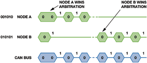
CAN 2.0b, which defines the implementation of the data-link layer, specifies the structure of CAN frames used for transmission. An arbitration field, which includes a message ID, starts the message. A lower message ID (more initial zeroes) will have higher priority, so the node is more likely to win arbitration when transmitting a message.
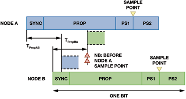
Although CAN nodes synchronise to the bus transmissions, two nodes that transmit together will not be exactly concurrent due to the propagation delay between them. For arbitration to work, the propagation delay must not be too large, or the faster node may sample the bus before detecting the bit state transmitted by the slower node. The worst-case propagation delay is twice the delay between the two furthest nodes. If nodes A and B in Figure 3 are the furthest apart on the bus, the critical parameter is the round trip time of TPropBA plus TPropBA.
The total propagation delay comprises the round trip time through the cable, two CAN controllers’ I/O and two CAN transceivers. The CAN controller I/O is not a major contributor, and can often be ignored, but a thorough assessment will allow for it. Loop time comprises the propagation delay from TxD to CANH/CANL and back to RxD. The cable propagation delay depends on the cable and distance, with 5 ns/m being a typical value.
At lower data rates, the allowed bit time is longer, so the propagation delay (and thus the cable distance) can also be longer. At the maximum standard CAN data rate of 1 Mbps, the allowed propagation delay is more limited, though ISO 11898-2 specifies a bus length of 40 m for operation at 1 Mbps.
Impact of isolation
With isolation, an extra element must be considered in the round trip propagation delay calculation. Digital isolators reduce the propagation delay compared to optocouplers, but even the fastest isolated CAN transceivers will be comparable to the slower non-isolated transceivers.
If the total allowable propagation delay remains the same, the maximum cable length will be shorter in isolated systems, but it may be possible to reconfigure the CAN controller to increase the total allowed propagation delay.
Compensating for propagation delay
To compensate for propagation delays added by longer buses or isolation, specific parameters related to timing and synchronisation must be set up for the CAN controller. When configuring the controller, instead of simply selecting a data rate, the designer must set the variables that dictate the bit time used by the controller.
The baud rate prescaler (BRP) for the oscillator or internal clock sets the time quantum (TQ), and the bit time is a multiple of TQ. The hardware selection of the oscillator, software configuration of the BRP and number of TQ per bit time set the data rate.
The controller’s bit time is broken into three or four segments as shown in Figure 3. The total number of TQ per bit time includes one for synchronisation, plus programmed numbers for propagation delay (PROP), phase segment 1 (PS1) and phase segment 2 (PS2). Sometimes PROP and PS1 are combined. Configuration adjusts the sample point to allow for propagation delay and resynchronisation.
Setting the sample point later in the bit time allows for longer propagation delays, but like the overall data rate, the sample point is dependent on other timing variables, each of which has its own restrictions. For example, the internal clock/oscillator may be fixed and only integer BRP and TQ numbers can be used. Thus, the ideal data rate required for a certain cable length may be impossible to achieve, so either the cable must be shortened or the data rate must be reduced.
Resynchronisation results in PS1 being lengthened or PS2 being shortened by the number of TQ specified by the synchronisation jump width (SJW), so PS2 can never be shorter than SJW. The number of TQ required for SJW depends on the clock tolerance of CAN controllers, with crystal oscillators typically allowing the minimum TQ for SJW and PS2.
Configuring a CAN controller
To achieve a robust network with reliable timing and synchronisation between nodes, the system must be able to tolerate the propagation delay with the chosen data rate and CAN-controller clock. If it this is not possible, the options are to reduce the data rate, shorten the bus or use a different CAN- controller clock rate. A three-step configuration process follows.
Step 1: Check clock and prescaler-match data rate
First check the possible configurations given the desired data rate and the CAN-controller clock. The TQ interval must be calculated based on the clock and various BRP values, and only the combinations where the TQ interval divides into the bit time by an integer number are possible.
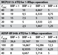
Depending on the system design stage, it may be possible to consider other CAN controller clock rates as well. Table 1 shows example calculations given a 1 Mbps maximum data rate using a Microchip MCP2515 standalone CAN controller and an ADSP-BF548 Blackfin processor with built-in CAN controller. The MCP2515 fOSC depends on the external hardware oscillator used, while the ADSP-BF548 fSCLK is determined by the hardware CLKIN and internal PLL settings (CLKIN multiplier for VCO, VCO divide-down for SCLK).
Only certain combinations of CAN controller clock and BRP (an integer number of TQ) will allow a 1 Mbps data rate, as shown in bold. This limits the settings for the bit timing, as only certain options are available once a bus data rate has been chosen.
Step 2: determine bit segment configuration
The next step is to determine the number of TQ required for each bit segment. The most difficult case is supporting the maximum propagation delay at a 1 Mbps data rate, with a 40 m cable and isolated nodes, for example. Ideally, the bit time segments should be configured so that the sample point is as late as possible in the bit.
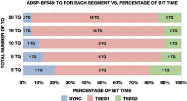
For each integer total number of TQ in Table 1, one TQ must be allowed for the SYNC segment, and the PS2 (or TSEG2) segment must be large to accommodate the CAN-controller information processing time (2 TQ for MCP2515, <1 TQ for ADSP-BF548 as long as BRP > 4). Also, for the MCP2515, PROP and PS1 can be 8 TQ maximum each; for the ADSP-BF548, TSEG1 (PROP + PS1) can be16 TQ maximum.
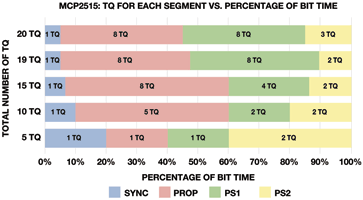
Figure 4 and Figure 5 show the possible total TQ configurations for MCP2515 and ADSP-BF548 respectively, with the latest sample point possible for the valid combinations of clock and BRP for 1 Mbps operation. The optimum total TQ for the MCP2515 is 19, requiring a hardware oscillator of 38 MHz and BRP of 1. For the ADSP-BF548, all the configurations except for a total of 5 TQ are at least 85% sample point, but the optimum setting is 10 TQ, requiring fSCLK = 50 MHz with BRP = 5.
Step 3: Match transceiver/isolation delay and bus length to configuration
Having achieved the optimum sample point for the CAN controller, the last step is to compare the allowable propagation delay with the CAN transceiver/isolation and bus length used. Assuming the ADSP-BF548 optimum configuration of 10 TQ (fSCLK = 50 MHz, BRP = 5), the maximum propagation delay possible is 900 ns.
For the ADM3053 isolated CAN transceiver with integrated isolated power, the data-sheet maximum loop delay (TxD off to receiver inactive) is 250 ns. This must be doubled (500 ns) to include both transmit and receive delays at two nodes at the furthest ends of the bus.
Assuming a 5 ns/m cable propagation delay, a bus length of 40 m (maximum for 1 Mbps per ISO 11898) could be accommodated with the ADSP-BF548 having a total of 10 TQ in bit time with only 1 TQ for the TSEG2 bit segment. In practice, slightly earlier sample points may suffice, as even an extreme transceiver propagation delay on one node would likely result in a simple retransmission (handled automatically by the CAN controller at the data-link layer), but the small delay between the CAN-controller I/O and the CAN transceiver makes it advisable to configure the sample point to the latest point possible.
Conclusion
Isolation adds robustness, but it will also add a propagation delay, in both transmit and receive directions. This delay must be doubled to account for two nodes in arbitration. If the allowed propagation delay in the system is fixed, then the cable length or data rate may be decreased if isolation is added.
An alternative is to reconfigure CAN controllers to allow the maximum possible propagation delay to ensure that the desired data rate and bus length are possible, even with isolated nodes.
For more information contact Arnold Perumal, Avnet South Africa, +27 (0)11 319 8600, [email protected], www.avnet.co.za


© Technews Publishing (Pty) Ltd | All Rights Reserved
 printer friendly version