


In the first article [March 2023, http://www.dataweek.co.za/18832r], it was shown how a classic linear program execution in a microcontroller differs from a CNN. The CIFAR network, with which it is possible to classify objects such as cats, houses, or bicycles in images, or to perform simple voice pattern recognition, was discussed. Part 2 explains how these neural networks can be trained to solve problems.
The training process for neural networks
The CIFAR network, which is discussed in the first part of the series, is made up of different layers of neurons, as shown in Figure 1. The image data from 32 pixels × 32 pixels are presented to the network and passed through the network layers. The first step in a CNN is to detect and investigate the unique features and structures of the objects to be differentiated. Filter matrices are used for this. Once a neural network such as the CIFAR has been modelled by a designer, these filter matrices are initially still undetermined, and the network at this stage is still unable to detect patterns and objects.
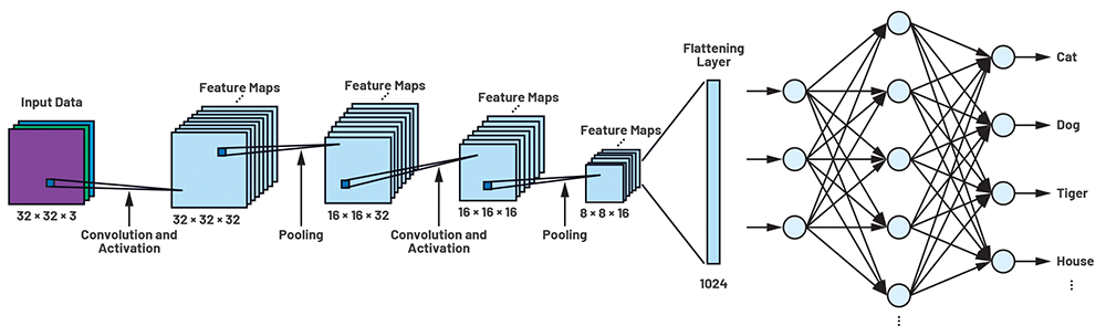 Figure 1. CIFAR CNN architecture.
To facilitate this, it is first necessary to determine all parameters and elements of the matrices to maximise the accuracy with which objects are detected, or to minimise the loss function. This process is known as neural network training. For common applications as described in the first part of this series, the networks are trained once during development and testing. After that, they are ready for use and the parameters no longer need to be adjusted. If the system is classifying familiar objects, no additional training is necessary. Training is only necessary when the system is required to classify completely new objects.
Training data is required to train a network, and later, a similar set of data is used to test the accuracy of the network. In our CIFAR-10 network dataset, the data are the set of images within the ten object classes: aeroplane, automobile, bird, cat, deer, dog, frog, horse, ship, and truck. However – and this is the most complicated part of the overall development of an AI application – these images must be named before training a CNN.
The training process works according to the principle of backpropagation; the network is shown numerous images in succession and simultaneously conveyed a target value each time. In our example, this value is the associated object class. Each time an image is shown, the filter matrices are optimised so that the target and actual values for the object class match. After this process has been completed, the network can also detect objects in images that it did not see during training.
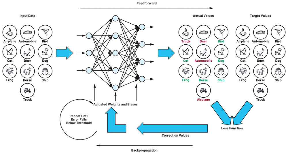 Figure 2. A training loop consisting of feedforward and backpropagation.
Overfitting and underfitting
In neural network modelling, questions often arise around how complex a neural network should be – that is, how many layers it should have, or how large its filter matrices should be. There is no easy answer to this question. In connection with this, it is important to discuss network overfitting and underfitting.
Overfitting is the result of an overly complex model with too many parameters. We can determine whether a prediction model fits the training data too poorly or too well by comparing the training data loss with the test data loss. If the loss is low during training and increases excessively when the network is presented with test data that it has never been shown before, this is a strong indication that the network has memorised the training data instead of generalising the pattern recognition. This mainly happens when the network has too much storage for parameters, or too many convolution layers. In this case, the network size should be reduced.
Loss function and training algorithms
Learning is done in two steps. In the first step, the network is shown an image, which is then processed by a network of neurons to generate an output vector. The highest value of the output vector represents the detected object class, like a dog in our example, which in the training case does not yet necessarily have to be correct. This step is referred to as feedforward.
The difference between the target and actual values arising at the output is referred to as the loss, and the associated function is the loss function. All elements and parameters of the network are included in the loss function. The goal of the neural network learning process is to define these parameters in such a way that the loss function is minimised. This minimisation is achieved through a process in which the deviation arising at the output (loss = target value minus actual value) is fed backward through all components of the network until it reaches the starting layer of the network. This part of the learning process is known as backpropagation.
A loop that determines the parameters of the filter matrices in a stepwise manner is thus yielded during the training process. This process of feedforward and backpropagation is repeated until the loss value drops below a previously defined value.
Optimisation algorithm, gradient, and gradient descent method
To illustrate our training process, Figure 3 shows a loss function consisting of just the two parameters x and y. The z-axis corresponds to the loss. The function itself does not play a role here and is used for illustration purposes only. If we look more closely at the three-dimensional function plot, we can see that the function has a global minimum as well as a local minimum.
A large number of numerical optimisation algorithms can be used to determine weights and biases. The simplest one is the gradient descent method. The gradient descent method is based on the idea of finding a path from a randomly chosen starting point in the loss function that leads to the global minimum, in a stepwise process using the gradient. The gradient, as a mathematical operator, describes the progression of a physical quantity. It delivers, at each point of our loss function, a vector – also known as a gradient vector – that points in the direction of the greatest change in the function value. The magnitude of the vector corresponds to the amount of change. In the function in Figure 3, the gradient vector would point toward the minimum at a point somewhere in the lower right (red arrow). The magnitude would be low due to the flatness of the surface. The situation would be different close to the peak in the further region. Here, the vector (green arrow) points steeply downward and has a large magnitude because the relief is large.
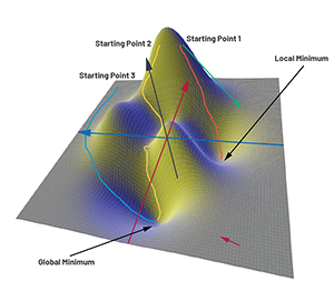
With the gradient descent method, the path that leads into the valley with the steepest descent is iteratively sought, starting from an arbitrarily chosen point. This means that the optimisation algorithm calculates the gradient at the starting point and takes a small step in the direction of the steepest descent. At this intermediate point, the gradient is recalculated and the path into the valley is continued. In this way, a path is created from the starting point to a point in the valley.
The problem here is that the starting point is not defined in advance but must be chosen at random. In our two-dimensional map, the attentive reader will place the starting point somewhere on the left side of the function plot. This will ensure that the end of the (for example, blue) path is at the global minimum. The other two paths (yellow and orange) are either much longer or end at a local minimum. Because the optimisation algorithm must optimise not just two parameters, but hundreds of thousands of parameters, it quickly becomes clear that the choice of the starting point can only be correct by chance. In practice, this approach does not appear to be helpful. This is because, depending on the selected starting point, the path and thus,the training time, may be long, or the target point may not be at the global minimum, in which case the network’s accuracy will be reduced.
As a result, numerous optimisation algorithms have been developed over the past few years to bypass the two problems described above. Some alternatives include the stochastic gradient descent method, momentum, AdaGrad, RMSProp, and Adam, to name a few. The algorithm that is used in practice is determined by the developer of the network because each algorithm has specific advantages and disadvantages.
Training data
As discussed, during the training process, we supply the network with images marked with the right object classes such as automobile, ship, etc. For our example, we used an already-existing CIFAR-10 dataset. In practice, AI may be applied beyond the recognition of cats, dogs, and automobiles. If a new application must be developed to detect the quality of screws during the manufacturing process, for example, then the network also has to be trained with training data from good and bad screws. Creating such a dataset can be extremely laborious and time-consuming and is often the most expensive step in developing an AI application.
Once the dataset has been compiled, it is divided up into training data and test data. The training data are used for training as previously described. The test data are used at the end of the development process to check the functionality of the trained network.
Conclusion
In the first part of this series a neural network was described and its design and functions were examined in detail. Now that all the required weights and biases for the function have been defined, it can be assumed that the network should work properly.
In the final article (part 3), our neural network for recognising cats will be tested by converting it into hardware. For this, the MAX78000 artificial intelligence microcontroller, with a hardware-based CNN accelerator developed by Analog Devices, will be used.
| Tel: | +27 11 923 9600 |
| Email: | [email protected] |
| www: | www.altronarrow.com |
| Articles: | More information and articles about Altron Arrow |


© Technews Publishing (Pty) Ltd | All Rights Reserved
 printer friendly version