


Ref: z263141m
SPICE simulations can model the characteristics of inductive components for lighting with high precision. The electrical parameters of ballasts for fluorescent lamps, for example, can thus be optimised. Epcos supplies accurate data for modelling inductive components.
Semiconductors have done much to make ballasts for fluorescent lamps more compact, efficient and long-lasting. Progress made in smart power ICs now make integration of protective elements and timers as well as field-effect power transistors possible. However, not all the risks involved in developing IC circuits for lighting applications have been banished, because some of the external components needed still cannot be reliably modelled. The transient analysis used in this process primarily requires faithful models of magnetic energy storage devices and realistic models of lamps.
For some time now, the simulation tool known as SPICE (simulation program with integrated circuit emphasis) has made it possible to include soft magnetic materials in simulations of entire circuits. Their characteristics are described in phenomenological terms by a few equations that provide considerable insight. Whereas circuits containing inductive components can often be simulated with astonishing accuracy, not all their properties can be perfectly simulated. However, developers are fully compensated for this weakness by the high degree of transparency of inductive components.
A few parameters suffice for simulation
SPICE uses the physical hysteresis model developed by D.C. Jiles and D.L. Atherton, which requires only a few parameters (Figure 2 and Figure 3) and whose set of formulas, based on a first-order differential equation, is relatively easy for computers to process.
The data required for an electrical model of a coil or transformer can be calculated from the magnetic form parameters and magnetisation of the soft magnetic material.
The energy stored in the magnetic field is defined in the following equation:
These formulas already contain the first two parameters of the Jiles-Atherton model, namely A and I. The values for effective magnetic cross-section Ae and effective magnetic path length Ie specified in the EPCOS data book for each ferrite core may be used directly in the model. SPICE performs its calculations in centimetres and square centimetres, so that the results must be converted accordingly.
The magnetic field inside the core is made up of the superimposed effects of magnetisation and magnetic field strength:
For ferrite materials, the value of the field parameter α in (3) fluctuates quite accurately around the number 10-4. α is not a model parameter in every SPICE implementation as it has a very limited influence on the model, so that it is assigned a standard value of 10-3 not optimum for ferrite materials in the following treatment. A core made of an isotropic material has a nonlinear magnetisation characteristic. It can be described as an approximation by the Langevin function:
The saturation magnetisation Ms can be easily obtained from the saturation flux density Bs.
Ms is a SPICE parameter. The graph of the Langevin function (5) is already comparable with the magnetisation curve specified in the material data sheet. The new curve can be compared with particular ease with that of the Langevin function at the transition to saturation. Variation of parameter α allows the Langevin function to be modified until it matches the function specified in the material data sheet.
The Jiles-Atherton model does not explicitly specify relative permeability µr. First, because it is transparent to the simulator via the Langevin function, and second, because this would reduce the accuracy of the simulation. The accuracy of the hysteresis model at low field strengths depends particularly on the precision with which the reversible magnetisation is specified. This parameter quantifies the degree of wall displacement of those domains whose spontaneous magnetisation lines up with the direction of the magnetic field. These displacements are reversible at low field strengths, whereas irreversible wall shifts determine the magnetisation in the steeper parts of the new curve.
The reversible magnetisation can be represented as the difference between magnetisation on the hysteresis loop and irreversible magnetisation. A proportionality factor c is introduced for this purpose:
The model parameter c is defined as the ratio of the susceptibility of the new curve to that of the hysteresis curve. In practice, however, it is more useful to divide the maximum amplitude permeability by the initial permeability (9).
The irreversible permeability can be determined from a differential equation of the first order with the aid of a computer according to the following formula:
The formula for dMirr/dH (10) contains the last material constant still missing, namely k. This constant quantifies the energy required for another wall displacement. The model operates directly with values of the coercive field strength taken from the data sheets.
SPICE does not offer a model for simulating gas discharge lamps. However, the lamp is the central component in the simulation of an electronic ballast and must be modelled as realistically as possible.
The characteristic gas discharge effects in a cold lamp can be simply described by a characteristic (1). If this characteristic can be modelled in a simulation, fundamental circuit topologies can be simulated. As a real lamp has an impedance curve that varies with frequency after ignition, a time domain model must take into account the different lamp states in the simulation of the characteristic.
To avoid burdening the model with superfluous detail, it may be assumed that the ignition voltage has already been reduced to about 500 V by preheating the electrodes. Although this means that the simulation of the right-hand part of the characteristic is somewhat skewed, only the preheating time is reduced. The lamp model described here (Figure 4) represents the right hand part of the characteristic of the voltage-controlled current source G_ion with the current/voltage curve shown in (Figure 5).
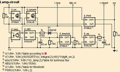
The elements E_ABS, R2, D1, C1, R3 and E_threshold as well as the current-controlled voltage source H_lamp are included so that the lamp can record the ignition. The absolute value of the voltage generated by H_lamp, which is proportional to the lamp current, charges the capacitor C1 via R2 and D1. If the voltage at C1 exceeds a threshold of 0,9 V, the voltage at the output of E_threshold changes from 0 to 1 V (node light_on). The lamp has ignited and changes suddenly from the left hand side of the characteristic (Figure 1) to its right-hand side into which the current source G_dynamic is connected. G_dynamic simulates the linear current/voltage characteristic between 10 mA and 1 A. Although a higher-order polynomial would have to be selected to simulate the overdrive response, such an operating condition makes no sense in reality because it would result in destruction of the lamp.
The equation formulated by M. Gulko and S. Ben-Yaakov for calculating the equivalent resistance of a fluorescent lamp is valid over the entire frequency range:
The lamp constants Vs, Rs can be determined experimentally by linearising the characteristic between 10 mA and 1 A. Typical Vs values for a 20 W lamp are found at 90 V and Rs values at 80 Ω.
Calculating the lamp current
Equation (11) applies to fluorescent lamps with constant RF excitation and a slow change in lamp output. In the event of a rapid increase in the lamp current, the charge carrier density rises after a significant delay, so that a higher ignition voltage is set up via several excitation cycles whose amplitude curve can be simulated with a low-pass filter of the first order.
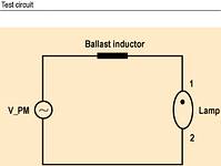
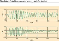
In the SPICE model presented here, the RMS value of the lamp current is calculated in the components E_sqr, R4, C2 and G_dynamic. E_sqr squares the lamp current converted by H_lamp into a voltage with a proportionality factor of 1, whereas R4 and C2 simulate the integral with a time constant R4•C2. To prevent the model from becoming unnecessarily large, the square-root operation is integrated into the calculation of G_dynamic. The test circuit shown in (Figure 6) and the result of the simulation in (Figure 7) illustrate the effect of the time constants R4•C2 on the lamp voltage. The voltage source V_PM is implemented so that it modulates the phase with a swing of 90°. The phase modulation of the operating frequency produces amplitude modulation of the lamp current because reactive impedance of the ballast inductance varies with frequency.
The effect of the carrier generation inertia on the modulation of the excitation frequency is shown in Figure 7. This frequency is phase-modulated with 500 Hz up to a simulation time of 4 ms, then with 1 kHz from 4 to 7 ms, 2 kHz from 7 to 10 ms and 5 kHz from 10 to 13 ms. At 200 Hz modulation, the carrier generation is fast enough for the lamp voltage to drop linearly according to (11) as the current rises. At 2 kHz, it is already obvious that the lamp voltage and current are in phase as they increase. The response of a real lamp corresponds to the simulation result, the linearisation of the characteristic in equation (11) making the greatest contribution to the divergence.
In addition to electrical simulation of a fluorescent lamp, the lamp model presented here has an output at which the luminous flux Φ (in lumens) is applied as a voltage. Φ = V(pwr) = f(V(1,2)·I(H_lamp))= 1 lumen/V. The average output voltage of E_PWR provides insight into the actual luminous flux.
Practical example of energy-saving lamps
The transformer and lamp model shown in Figure 8 is typically used in energy-saving lamps of low output. The generator circuit oscillates freely after ignition of lamp U2. To excite the circuit before the lamp ignites, brief pulses must be impressed on the gate of M2. This part of the circuit was left out for the sake of simplicity.
In the simplest case, it is sufficient to discharge a capacitor repeatedly by means of a trigger diode (Diac) via L4 and R4. In continuous operation, the half-bridge (M1, M2) generates a square-wave oscillation whose frequency f is determined by the components L5, C1 and L4, C2. The resonant circuits L5, C1 and L4, C2 are then excited with a phase shift of exactly 180° via the transformer windings L1 and L3.
L4 and L5 correspond to RF choke B78108-S1475-J from Epcos. R1 and R2 are designed so that only the energy lost in the resonant circuits at the gates of M1 and M2 is subsequently recharged. The current flowing through the fluorescent lamp U2 is limited by the lamp choke L2. C3 eliminates the DC component, whereas C4 is used only during the ignition phase as a resonant circuit capacitor. R5 and R6 are used to simulate the heating coil. R7 is preferably implemented with a PTC thermistor to load the resonant circuit C4, L2 during the heating phase and thus heat up the heating coils R5 and R6 to operating temperature.
The transformer TX1 can be implemented with a ferrite core of type EF16. Ferrite materials N27 and N67 (Figure 3) are suitable core materials, with an inductance factor AL of 85 nH (air gap approximately 0,37 mm). The two graphs in Figure 9 depict the key electrical parameters of Figure 8 during ignition and shortly afterward. V(LC) is the curve of the lamp voltage, referred to the supply voltage. The upper graph shows the magnetic flux density in the core B(TX1). To show this in teslas, the values output in gauss by PROBE must be divided by 10 000.
Data helps design
The models can be used to reliably simulate energy saving lamps and electronic ballasts. This considerably facilitates the design of integrated circuits for lighting applications.
Epcos has built up a wealth of data on the properties and performance of inductive components. With the theories described above, this database is used to develop inductive components optimised to customer requirements. Thanks to realistic description of the properties of the principal external passive components, the risk of design errors in the development of monolithically integrated circuits can be minimised. Epcos develops and manufactures lamp chokes and resonant chokes with ferrite core types E16 to E32, EFD25 and EV30. Using the tools and know-how presented here, Epcos can develop customer-specific transformers that perfectly match the ICs used and thus produce lamp ballasts of optimum design and economy.
In summary
SPICE simulations with inductive components offer key design benefits:
* Congruence of simulation and real operation for one-shot design
* Few parameters required
* Precise data is available in EPCOS documentation
| Tel: | +27 11 458 9000 |
| Email: | [email protected] |
| www: | www.electrocomp.co.za |
| Articles: | More information and articles about Electrocomp |


© Technews Publishing (Pty) Ltd | All Rights Reserved
 printer friendly version